

Abstract
Global hydrological models (GHMs) supply key information for stakeholders and policymakers simulating past, present and future water cycles. Inaccuracy in GHM simulations, i.e. simulation results that poorly match observations, leads to uncertainty that hinders valuable decision support. Improved parameter estimation is one key to more accurate simulations of global models. Here, we introduce an efficient and transparent way to understand the parameter control of GHMs to advance parameter estimation using global sensitivity analysis (GSA). In our analysis, we use the GHM WaterGAP3 and find that the most influential parameters in 50% of 347 basins worldwide are model parameters that have traditionally not been included when calibrating this model. Parameter importance varies in space and between metrics. For example, a parameter that controls groundwater flow velocity is influential on signatures related to the flow duration curve but not on traditional statistical metrics. Parameters linked to evapotranspiration and high flows exhibit unexpected behaviour, i.e. a parameter defining potential evapotranspiration influences high flows more than other parameters we would have expected to be relevant. This unexpected behaviour suggests that the model structure could be improved. We also find that basin attributes explain the spatial variability of parameter importance better than Köppen–Geiger climate zones. Overall, our results demonstrate that GSA can effectively inform parameter estimation in GHMs and guide the improvement of the model structure. Thus, using GSA to advance parameter estimation supports more accurate simulations of the global water cycle and more robust information for stakeholders and policymakers.
Export citation and abstract BibTeX RIS

Original content from this work may be used under the terms of the Creative Commons Attribution 4.0 license. Any further distribution of this work must maintain attribution to the author(s) and the title of the work, journal citation and DOI.
1. Introduction
Global hydrological models (GHMs) are used to simulate and assess past, current and future water availability and to estimate hydrological extremes (e.g. Krysanova et al 2017, Zaherpour et al 2018, 2019, Schewe et al 2019, Boulange et al 2021, Satoh et al 2022). Their simulations underpin guidance for international policy related to floods, drought, and water resources management. Moreover, the results of GHMs are used for further analyses in an even broader context, e.g. to analyse the effects of food trade (Soligno et al 2019) or in the field of ecosystem health (Liu et al 2021).
GHMs often exhibit a limited ability to match observations (van Loon et al 2012, Beck et al 2017, Zaherpour et al 2018, Schewe et al 2019), which weakens the value of modelling results (Krysanova et al 2020). Several approaches exist to increase the model's accuracy. For example, changing the model structure, i.e. the basic model equations that display the underlying perceptual concept of the model, or changing the parameters 'that define the characteristics of the catchment area' (Beven 2008). For GHMs, past efforts have largely focused on such model structure improvement, e.g. by comparing results of different models in multi-model studies or by including additional or alternative processes within the model (e.g. Verzano et al 2012, Zhao et al 2017, Veldkamp et al 2018). Uncertainty in parameter estimates has rarely been addressed, even though it is expected to be high (van Loon et al 2012, Luo and Schuur 2020).
Calibration is the process of adjusting parameter values to achieve the best match between model simulations and observations. This match is often far from optimal when using a priori parameter estimates (Beven 2008). Most GHMs are not calibrated (van Loon et al 2012, Müller Schmied et al 2014, Yoshida et al 2022), i.e. parameter estimates are a priori derived using empirical equations (e.g. Cuntz et al 2016) or directly from hydrogeological or vegetation attributes (Duan et al 2001). One problem with linking parameter values directly to measurements is that model parameters and measurements typically refer to different scales. For example, land use or soil characteristics are used in GHMs as aggregated mean values per grid cell, neglecting the spatial variability within each grid cell. In addition, the issue of equifinality (Beven 2006) and the challenge of transparency (Hutton et al 2016) are often ignored. In recent years the community recognised the need to improve parameter estimation methods for GHMs (Bierkens 2015, Beck et al 2017, Samaniego et al 2017).
Several obstacles exist when estimating parameters for GHMs. (1) The number of parameters in GHMs is usually quite high, e.g. the GHM World-wide Hype (Arheimer et al 2020) requires twenty-two parameters for snow and soil processes in each grid cell, even when disregarding routing and evapotranspiration parameters (Santos et al 2022). Such complexity means that a very large space has to be searched for optimal parameter values, leading to high information need for parameter estimation (Gupta et al 2008). (2) GHMs demand immense computational power (Yoshida et al 2022). Thus, an efficient parameter estimation strategy is needed. (3) Basins are highly diverse over the globe (Kuentz et al 2017, Addor et al 2018), and influential parameters are likely to vary (e.g. Rosero et al 2010, Mai et al 2022).
In the history of GHMs, these obstacles were often tackled using expert knowledge to avoid extensive model calibration. To account for systematic differences between basins, climate zones such as Köppen–Geiger are usually used (e.g. Chaney et al 2015, Zaherpour et al 2018, van Kempen et al 2021, Yoshida et al 2022). Lately, some effort has been made to develop effective calibration frameworks suitable for GHMs (Beck et al 2020, Schweppe et al 2021, Yoshida et al 2022), integrating climate or basin information within the automated calibration process. Most of these studies were made to obtain hydrologically meaningful parameter sets. However, parameter sensitivity, i.e. whether a parameter is influential for a specific model output or metric, has rarely been addressed, leaving space for the choice of calibration parameters. However, understanding dominant model parameters and their variability in space is indispensable to ensure that parameter estimation is effective and tailored towards global model applications. Thus, enhancing the knowledge about parameter control increases confidence in getting the right answers for the right reasons (Kirchner 2006).
Global sensitivity analysis (GSA) is a powerful tool for parameter estimation and model evaluation (Pianosi et al 2016, Saltelli et al 2020, Razavi et al 2021). In contrast to local sensitivity analysis, GSA allows the investigation of the entire parameter space and not only around a baseline parameter set. GSA can detect uninfluential parameters that can be excluded from computationally-expensive calibration (Bastidas et al 1999, Muleta and Nicklow 2005, Cuntz et al 2015, Markstrom et al 2016). Further, parameter sensitivity can be linked with physical basin characteristics to enhance process understanding (Demaria et al 2007, van Werkhoven et al 2008), which can be included in parameter estimation in both gauged and ungauged situations. Additionally, 'internal consistency' (Wagener and Pianosi 2019, Wagener et al 2022) can be tested to ensure that the model structure represents the underlying assumptions of the described hydrological processes in line with the modeller's intentions. Internal consistency is especially important for GHMs as they are often applied for scenario analysis without validation data.
In recent years, increasing computational power has enabled applying well-known techniques for parameter estimation to GHMs (Arheimer et al 2020). GSA has also been used for GHMs to guide future model development, i.e. detecting influential modelling parts to focus model development (Rosero et al 2010, Gosling and Arnell 2011, Chaney et al 2015). Furthermore, GSA has guided parameter estimation, i.e. detecting influential parameters to simplify calibration (Cuntz et al 2016, Zajac et al 2017, Reinecke et al 2019). Additionally, Santos et al (2022) applied GSA to link overall model performance and parameter values to Köppen–Geiger climate zones to highlight advantages for model calibration and regionalisation for the GHM World-wide Hype. However, technical constraints still pose challenges for applying GSA (Santos et al 2022), e.g. model parameters are hard-coded (Cuntz et al 2016), and input and output handling is cumbersome.
This study addresses the parameter estimation problem for a highly popular GHM by applying GSA to a new lightweight model version of WaterGAP3 (Schneider et al 2011, Flörke et al 2018, Müller Schmied et al 2021) using multiple streamflow criteria. We use GSA to screen the parameters' importance to guide the selection of parameters and evaluation criteria, e.g. as a basis for efficient model calibration. Moreover, combining these results with basin characteristics increases our knowledge of parameter control. Additionally, comparing these findings with the underlying perceptual model (Beven 2008) enables us to review the 'internal consistency' of WaterGAP3. The gained knowledge leads to a better understanding of processes in WaterGAP3, which is indispensable for model improvement. To tackle the technical constraints of WaterGAP3, we introduce the re-coded model version, WaterGAPLite, enabling GSA's efficient and effective application.
2. Data and methods
2.1. Model
WaterGAPLite (2023) is a lightweight version of the established GHM WaterGAP3. The revised model is fully distributed and simulates basin-wise the terrestrial water cycle on a five-arcminute grid with a daily resolution. In contrast to the original model version that is written in C/C++, WaterGAPLite is written in R/Rcpp, enabling more flexible handling of I/O data and model parameters, thus, facilitating the application of GSA. The rewritten code offers higher readability leading to more transparency. The code is freely available on GitHub under the GNU General Public License, Version 3. The supplementary information (SI) and the GitHub repository provide a detailed explanation of the model structure.
The standard WaterGAP3 input (Schneider et al 2011) with updated soil and land use information is used to run the model. The settings demanding water use estimates are not considered to focus on the uncertainty in model parameters and structure for WaterGAP3. Thus, water use is set to zero, and reservoirs that rely on such estimates are treated as lakes. These settings ensure that uncertainty related to the water use model is not affecting the analysis of the hydrological model WaterGAP3. In contrast to traditional model runs, streamflow velocity is used as a time-invariant parameter because the alternative option of variable calculation only considers the effects of routing but not yet flooding effects (Verzano et al 2012). In total, 17 model parameters are investigated (see table S1). Traditionally, only a single parameter (γ) would be calibrated in WaterGAP3. This parameter mainly controls how much water is released from the soil, thus influencing flow volume and variation. The role of each investigated model parameter within the model is explained further in the supplement.
2.2. Data
We use the EWEMBI dataset (Lange 2016), which was compiled to support the bias correction of climate input data for the multi-model study ISIMIP. As streamflow data, we use the complete dataset from the Global Runoff Data Centre 56 068 Koblenz, Germany (GRDC) from 2020. The simulation period is from 01.01.1980 to 01.01.1990, which is the period with the most station data available in the GRDC catalogue (see figure S1). To select adequate gauging stations, we applied several criteria: (1) a basin size > 5000 km2, (2) unnested basins, and (3) the basin size fits the five-arcminute model grid with less than 30% of deviation. A total of 740 gauging stations meet the criteria and are used in this study (see figure S2). Of these 740 stations, 347 were defined as 'stations with sufficient streamflow quality'. These are stations (1) containing more than five years of streamflow data between 1980 and 1990, (2) with an amount of streamflow that is smaller than the amount of precipitation, and (3) with streamflow that exceeds minimal correlation to precipitation. For these stations, the gauged streamflow data is used to calculate statistical metrics. For the other stations, only metrics based on the simulated streamflow are calculated and used for the GSA. Here, we assume that ten years are long enough to represent the basins' climate. Due to the limited data availability of observed streamflow, no additional period is used.
Köppen–Geiger climate zones from Kottek et al (2006) are used to analyse systematic patterns between basins and parameter influence. In addition, meteorological and geohydrological information is used to detect relationships between parameter influence and basin attributes. We use correlation coefficients and apply Random Forest to detect systematic patterns between parameter importance and basin information. A full overview of the used basin attributes and their variety is provided in the SI (see figure S6).
2.3. Morris methods and evaluation metrics
We apply the Morris Method (Morris 1991) to estimate the sensitivity of different evaluation metrics to model parameters. The Morris Method is a well-established GSA that is computationally very efficient (Campolongo et al 2007) and has already been used at the global scale (Reinecke et al 2019). The method starts by generating a random sample of n 'baseline' points in the parameter space, which is the space between all parameters' lower and upper bounds. Then, for each baseline point, it calculates each parameter's elementary effects (EEs) as the finite difference in the output (e.g. an evaluation metric) when perturbing that parameter by a fixed amount Δ. For each parameter, the mean of the absolute EEs (denoted by µ*) across the baseline points is taken as a measure of the total effect of that parameter. The higher µ*, the more important the parameter, and the lower its rank number (i.e. 1 is top in the ranking). In our application, each parameter gets a rank for each metric and each basin. See the supplement for more information on the Morris Method and its settings.
As statistical metrics, we apply four well-established objective functions for model calibration. These are the Kling–Gupta efficiency (Gupta et al 2009), the Nash–Sutcliff efficiency (NSE) (Nash and Sutcliffe 1970), a logarithmic version of the NSE (logNSE) and the Pearson correlation coefficient (r). These metrics are calculated for the 347 stations with sufficient quality in observed streamflow to quantify the differences between simulated and observed daily streamflow. Additionally, we use signature-based metrics (Gupta et al 2008) to extract information regarding high, low, and average streamflow. Signature-based metrics exploit streamflow information and can improve calibration (Wagener et al 2009, Pfannerstill et al 2014, Shafii and Tolson 2015). We use a set of eight signature-based metrics, which are easy to compute and interpret (see SI for formulas). These are calculated for all 740 basins.
3. Results and discussion
3.1. Parameter influence on NSE
In hydrology, the NSE is probably the most popular metric for calibration (Schaefli and Gupta 2007, Gupta and Kling 2011). It is also used to evaluate GHMs' performance (e.g. Krysanova et al 2020, Müller Schmied et al 2021, Yoshida et al 2022). Therefore, we use the NSE to give a first overview of worldwide parameter importance in figure 1. Figure 1 displays the most influential parameter on the NSE for the examined 347 basins with sufficient streamflow and reveals that the importance of parameters changes from basin to basin. The standard calibration parameter for WaterGAP3, γ, is the most influential in only about 50% of the basins. In the remaining 50%, the influence of other parameters exceeds that of γ. Accordingly, calibrating the single parameter γ is not the best decision for 50% of all basins.
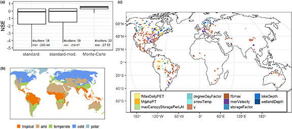
Figure 1. (a) NSE values for daily streamflow (1980–1990) for different calibration methods at 347 GRDC stations. Outliers (smaller 75th percentile + 1.5 IQR) are excluded, but information (number and minimum) is given. (b) Overview of the worldwide distribution of Köppen–Geiger climate zones. (c) Most influential parameter on NSE for the 347 basins.
Download figure:
Standard image High-resolution imageFor example, in colder regions like the northern parts of North America, snow parameters are more influential than γ. Similarly, in basins dominated by water bodies, like in the Great Lakes region in North America or the Nordic countries, water body parameters are more influential than γ. In the Amazon basin, a parameter that determines the size of interception storage (maxCanopyStoragePerLAI) is often the most influential.
Because the most important parameter on the NSE varies between basins, we want to highlight the potential of multivariate parameter estimation. Therefore, we apply a widely used multivariate parameter estimation strategy (Monte-Carlo simulation assuming independent uniform parameter distributions, 1000 simulation runs, Latin hypercube sampling) in contrast to the standard calibration, where solely γ is varied between 0.1 and 5. Subsequently, we compare the highest NSE per basin from the Monte-Carlo run with those derived by the standard calibration for all 347 basins with sufficient streamflow quality. Because in the standard calibration of WaterGAP3, the objective is to match the mean annual flow, we change the objective function to NSE in an additional calibration run to eliminate the effect of different objective functions. The best NSE for all three methods is shown in figure 1(a).
Figure 1(a) shows that the multivariate method outperforms the two standard methods using single parameter-based calibration. The number of outliers in the plot demonstrates that despite the carefully selected basins, there are still basins where the model structure needs to be improved or data quality needs to be higher. Although the Monte-Carlo simulation outperforms the standard calibration, this method is too computationally demanding as a parameter estimation strategy for GHMs: The standard calibration regularly uses ten simulation runs per basin, whereas the Monte-Carlo approach takes 1000 simulation runs. However, it demonstrates the potential of multivariate calibration for WaterGAP3.
3.2. Parameter influence and correlation
In figure 2(a), we show that the most influential parameter varies not only from basin to basin but also depends on the chosen metric. Figure 2(a) displays the parameter ranks (averaged across basins) based on the sensitivity measure µ* for each metric, i.e. lower ranks indicating higher importance. The six most influential parameters among all basins are highlighted in red (in fact, for guiding future parameter estimation, it is not important to know all ranks but to identify the subset of the most influential parameter). In some cases, the mean rank is not representative due to high variability within the ranks (see figure S7). Hence, these cases are disregarded and shaded in grey.

Figure 2. (a) Parameter ranks (average across basins) for each parameter (vertical) and metric (horizontal). The lower the number, the higher the position in the ranking, i.e. the more influential the parameter. Where variability of ranks across basins is too high, i.e. IQR > 6, results are deemed not representative, and boxes are shaded in grey. (b) Parameter ranks for NSE against attribute values for the most correlated attribute, using Spearman rank correlation for the definition of highest correlation.
Download figure:
Standard image High-resolution imageWithin the set of examined parameters, five parameters (namely evapoReductionExp, wetOutflowExp, lakeOutflowExp, runoffFracBuiltUp, and canopyEvapoExp) are generally uninfluential (see figure 2(a)). These parameters are either consistently at the bottom of the ranking (i.e. low variability across basins and a high mean rank, see figure S7(c)) or are rarely ranked top (i.e. high variability across basins and too few occurrences of low ranks, see figure S7(a)). Two parameters (γ, fSmax) are top-ranked in all metrics, indicating that they should always be carefully estimated. Both parameters are related to soil storage. Where γ is handling the release of water from the soil, the multiplier fSmax determines the size of the soil storage.
The parameter k_g that controls the groundwater flow velocity is top-ranked for low flow-related metrics (Q90, minTiming, FDC slope). The routing parameter riverVelocity, which controls the flow velocity in river segments, is most influential for streamflow timing (r). Thus, adding low-flow signatures and timing metrics to the set of metrics used for parameter estimation would enable better estimation of these two influential parameters. The use of additional streamflow signatures for model calibration is in line with van Werkhoven et al (2009) for basin scale models. The varying parameter importance for different evaluation criteria also underpins that purpose-dependent parameter estimation is beneficial (Janssen and Heuberger 1995). For example, parameter estimation should focus on high flow instead of the overall flow regime if a model is applied for flood management (e.g. Mizukami et al 2019).
Figure 2(a) also reveals some surprises. When focusing on the high flow related metric Q10, the multiplier for increasing potential evapotranspiration (fAlphaPT) is the 3rd most important parameter (in 58% of all basins in the top 3). In contrast, the storage constant for the routing parameter (riverVelocity) is only the 7th most influential parameter. However, in GHMs, the routing significantly impacts high flow peaks (Zhao et al 2017). This unexpected behaviour may point to structural errors in the solely storage-driven generation of fast runoff during high flow and needs further analysis.
Parameters related to snow and water bodies exhibit high variability in ranks across basins, as shown by the high number of grey-shaded boxes for these parameters in figure 2(a). This variability in the parameter importance can be explained by the variance in snow and water body occurrence, respectively. Figure 2(b) shows for these parameters (namely wetlandDepth, lakeDepth, storageFactor, snowTemp, degreeDayFactor) the parameter ranks of all basins against the basin attribute with the strongest Spearman rank correlation to the parameter ranks, exemplary for the NSE. Additionally, the Pearson correlation is displayed in figure 2(b) to quantify the linearity of the displayed relation.
The parameter ranks of the wetlandDepth display the strongest non-linear correlation within all parameter ranks. The corresponding Spearman rank correlation coefficient to the occurrence of wetlands is −0.963, i.e. the more wetlands, the more influential the wetlandDepth. Also, lakeDepth and storageFactor exhibit high Spearman rank correlation coefficients to lake fraction and global water body fraction, respectively.
For snow parameters (snowTemp, degreeDayFactor), the difference between Spearman rank correlation and Pearson correlation is minor, indicating a linear relationship between the associated attributes. For the snowTemp, the mean temperature displays the strongest correlation (−0.798) to the parameter ranks of the NSE. With decreasing mean temperature, the snowTemp becomes more influential for a basin. The parameter ranks of the degreeDayFactor exhibit a similarly strong correlation to the number of snow days, i.e. the more snow days occur, the more influential the degreeDayFactor.
Surprisingly, the dryness index does not correlate highly to any water body parameter (max. Spearman rank correlation: −0.362). In fact, there is no strong correlation between the dryness index and parameter ranks for any metric (max. Spearman rank correlation: 0.455). Thus, the dryness index does not exhibit a striking correlation related to parameter sensitivity, as found in previous studies (van Werkhoven et al 2008). This unexpected finding could be related to the direct integration of water bodies within WaterGAP3, which covers humidity's role. The correlation between humidity and evapotranspiration parameters might be higher without explicitly considering water bodies within the model structure.
Attributes related to soil properties (e.g. soil texture) do not exhibit any strong correlation (max. Spearman rank correlation: −0.400). Thus no systematic relation between soil properties and parameter sensitivity exists, which is in line with previous findings (e.g. Merz and Blöschl 2004, Addor et al 2018).
Because we use a globally applicable parameter space, the parameter ranges are quite wide, often resulting in wide ranges of model performance. The global parameter space, mainly derived from a literature review, is beneficial to make as few a priori assumptions as possible regarding basins and expected parameter behaviour. Thus, it enables us to analyse relationships as objectively as possible. However, a drawback is that parameter sets with very low model performance may influence our results. To check the robustness of our results, we conduct an additional analysis (see SI) for a better-performing subset of basins.
3.3. Linking parameter influence with basin attributes
To inform parameter estimation of GHMs, it is rather useful to split the parameters into two sets: important (which should be subject to calibration) and unimportant (which can be excluded by calibration). Knowing this distinction is more important than knowing the exact parameter rank for practical purposes. Assuming we want to calibrate parameters with a multi-objective approach (following van Werkhoven et al 2009) in a later stage, we determine if a parameter is important for calibration using the ranks of three different metrics (namely NSE, r, and Q90). Thus, a parameter is defined as 'important' if one of the three ranks is in the top 4. This procedure results in approximately six important parameters per basin, which is expected to be a feasible calibration load for WaterGAP3.
In figure 3, we examine whether using correlated attributes to distinguish important and unimportant parameters is more beneficial than using Köppen–Geiger climate regions. For this purpose, the basins are split into 50% testing and 50% training dataset. We train two decision trees (for further information on the decision tree set-up, see SI) to predict the importance of each parameter. One decision tree uses the Köppen–Geiger regions. The other uses the correlated attributes highlighted in figure 3(b) (namely lake fraction, wetland fraction, global water body fraction, mean temperature, and #snowDays). These correlated attributes were selected because they display the strongest systematic relation to parameter ranks.
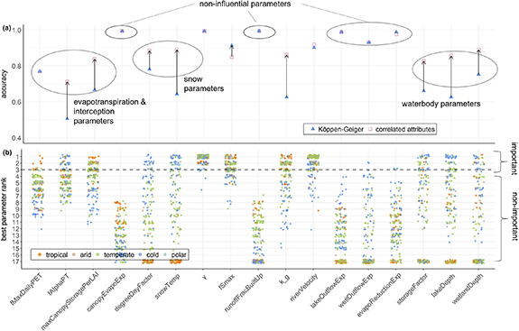
Figure 3. (a) Accuracy of decision trees to predict parameter importance and (b) corresponding best parameter rank (out of NSE, Q90 and r) used to define parameter importance and Köppen–Geiger climate zones per basin.
Download figure:
Standard image High-resolution imageFigure 3(a) shows the 'overall accuracy' (Congalton 1991) for the classification from the decision trees for each parameter using the test dataset: The higher the accuracy, the better the prediction of whether a parameter is important. In this figure, the correlated attributes outperform Köppen–Geiger regions to predict parameter importance. The decision trees using correlated attributes display equal or higher accuracy for all parameters than those using Köppen–Geiger information. The highest differences in accuracy are found for parameters related to water bodies and snow. Figure 3(b) shows the best parameter rank from the used metrics. (NSE, r, Q90) for the test dataset, coloured by the dominant Köppen–Geiger region. In this figure, it is striking that Köppen–Geiger regions do not exhibit clear systematics regarding parameter importance for most parameters, which results in lower performance for importance prediction (see figure 3(a)). Thus, the parameter importance, especially for parameters related to snow and water bodies, is more easily predicted using explicit information (e.g. more snow days lead to a stronger influence of snow parameters) than implicit information (e.g. in cold and polar regions, it is more likely that snow occurs and, thus, that snow parameters are influential).
The parameter importance for the groundwater-related parameter (k_g) is also predicted better using the correlated attributes. Further inspection of the decision tree of correlated attributes reveals that the tree uses wetland and lake occurrence to predict the parameter importance: if the lake and wetland fraction is high, k_g is classified as unimportant. This relation can be explained by the dampening effect of lakes and wetlands, which is especially visible in dry periods where the flow from groundwater dominates. Thus, with an increasing fraction of wetlands and lakes, k_g becomes less important. For uninfluential parameters (i.e. consistently unimportant parameters across almost all catchments), Köppen–Geiger regions and correlated attributes work equally well. For consistently important parameters (γ, fSmax), the Köppen–Geiger regions slightly outperform the correlated attributes in the case of fSmax. Whereas the decision tree of correlated attributes uses only the mean temperature to predict parameter importance regarding fSmax, the Köppen–Geiger regions are defined using mean temperature and mean annual discharge. The better performance of Köppen–Geiger climate zones indicates that the mean annual discharge might be useful information to integrate into the decision tree of correlated attributes to predict the parameter importance of fSmax. Overall, it is shown that correlated attributes outperform Köppen–Geiger regions in predicting parameter importance. Thus, considering (correlated) basin attributes or flow signatures to define similar hydrological regions (e.g. Kuentz et al 2017) might be a more beneficial approach to selecting parameters for parameter estimation than using climate zones, such as Köppen–Geiger.
3.4. Guidance towards parameter estimation
Our study contributes to a better understanding of model parameters in WaterGAP3 and enables an objective selection of parameters and evaluation criteria for parameter estimation. However, model performance for basins with sufficient streamflow quality exhibits distinct behaviour in our study. Mainly, these basins can be separated into two groups: (1) basins where parameter estimation is likely beneficial and (2) where not (see figure 4). Meaning that model performance is either high due to changes in parameter values or permanently low, disregarding changes in parameter values.

Figure 4. Conceptual distribution types of NSE values in Monte-Carlo simulation and counted basins per type in basin set. (Here, low variance is defined when the spread between the 90th and 10th percentile is smaller than 0.5. Low performance means that the maximal NSE value is lower than 0.25.) The full set of NSE values for all basins can be found in the SI (see figure S13).
Download figure:
Standard image High-resolution image
For a high proportion of the basins with sufficient streamflow quality, the model performance indicates that parameter estimation is beneficial to enhance model performance (269 out of 347). For basins with permanently low model performance (78 out of 347), parameter estimation would not be beneficial. Thus, these basins should not be part of parameter estimation to avoid that parameter estimation accounts primarily for deficiencies in the data or the model structure. Instead, it needs further research to understand the drivers for the permanently low model performance in these basins. Likely, other GHMs encounter similar issues (e.g. see figure 8 in Stacke and Hagemann (2021)), and acknowledging these knowledge gaps is indispensable for advances in large-scale modelling (Wagener et al 2021).
Furthermore, there are basins where varying model parameters have little influence on the model's performance (45 out of 347), indicating that parameters do not dominate the model performance but other issues. Using default parameter values instead of computationally demanding parameter estimation techniques for these basins could be beneficial.
4. Conclusion
GHMs supply key information to international stakeholders and policymakers. Accurate simulation results from GHMs are indispensable for meaningful decisions. However, GHMs' accuracy still needs improvement. New code structures and increasing computational power offer the opportunity to enhance model parameter estimation—a key to accurate simulations. Here, we introduce an efficient and transparent way to understand the parameter control of a GHM with the ultimate aim of advancing parameter estimation.
Utilising a computationally frugal GSA approach, our method is especially appealing for GHMs because it tackles three main obstacles. (1) Detecting uninfluential parameters enables more efficient parameter estimation, thus reducing the computational burden. (2) Integrating additional metrics better exploits the available information in streamflow and permits estimating more parameters. (3) Analysing systematic patterns in parameter influence increases the understanding of process representation through the model.
Our results show that the most influential parameter for 50% of 374 worldwide basins is not traditionally used for calibration, suggesting a need to improve parameter estimation for WaterGAP3. Furthermore, comparing the standard single parameter-based calibration approach with a multivariate technique reveal a big potential for simulation improvement for WaterGAP3. Parameter influence varies between metrics, and using multi-criteria calibration, e.g. including low flow-related metrics or using purpose-dependent calibration, may be beneficial for model calibration. Systematic patterns between parameter influence and basin attribute exist for parameters related to snow and water bodies. These systematic relations outperform traditionally used Köppen–Geiger climates zones for estimating influential and uninfluential parameters for worldwide basins. The GSA results also indicate structural errors may exist within WaterGAP3 regarding high flows and evapotranspiration. The results of an additional Monte-Carlo simulation reveal that regions exist where the model structure or the data quality is insufficient to reproduce historic streamflow.
Next, regions with permanently low model performance should be examined to attribute potential causes. Within this context, the model structure related to high flow and evapotranspiration should be revised to ensure internal consistency. Subsequently, the information gained on parameter importance and its relation to evaluation criteria and basin attributes can be used to improve parameter estimation for basins with adequate model structure and data quality, e.g. by application of a multivariate calibration routine based on our findings (e.g. using the PEST algorithm (Doherty et al 2010) or other efficient calibration strategies).
Acknowledgments
Funding for R R and T W has been provided by the Alexander von Humboldt Foundation in the framework of the Alexander von Humboldt Professorship endowed by the German Federal Ministry of Education and Research. F P was partially funded by the UK Engineering and Physical Sciences Research Council (EPSRC) though a 'Living with Environmental Uncertainty' Fellowship (EP/R007330/1).
J K had the idea, designed the experiment, conducted the experiment and did the writing. R R helped to design the experiment and analyse the results, and R R commented on the manuscript. T W and F P supported analysing the results and commented on the manuscript. M F commented on the manuscript.
Data availability statement
The model WaterGAPLite is available under the GNU General Public License v3.0 at GitHub (https://github.com/JKupzig/WaterGAPLite, Kupzig 2023).
The data that support the findings of this study are openly available at the following URL/DOI: 10.5281/zenodo.7906116.
Supplementary data (7.0 MB PDF)
Table of Parameter Importance (1.0 MB XLSX) The file show ranks of parameter importance for each metric using all examined basins. Furthermore, it overviews examined basin attributes for all 740 basins.