

Abstract
The BlueFlux field campaign, supported by NASA's Carbon Monitoring System, will develop prototype blue carbon products to inform coastal carbon management. While blue carbon has been suggested as a nature-based climate solution (NBS) to remove carbon dioxide (CO2) from the atmosphere, these ecosystems also release additional greenhouse gases (GHGs) such as methane (CH4) and are sensitive to disturbances including hurricanes and sea-level rise. To understand blue carbon as an NBS, BlueFlux is conducting multi-scale measurements of CO2 and CH4 fluxes across coastal landscapes, combined with long-term carbon burial, in Southern Florida using chambers, flux towers, and aircraft combined with remote-sensing observations for regional upscaling. During the first deployment in April 2022, CO2 uptake and CH4 emissions across the Everglades National Park averaged −4.9 ± 4.7 μmol CO2 m−2 s−1 and 19.8 ± 41.1 nmol CH4 m−2 s−1, respectively. When scaled to the region, mangrove CH4 emissions offset the mangrove CO2 uptake by about 5% (assuming a 100 year CH4 global warming potential of 28), leading to total net uptake of 31.8 Tg CO2-eq y−1. Subsequent field campaigns will measure diurnal and seasonal changes in emissions and integrate measurements of long-term carbon burial to develop comprehensive annual and long-term GHG budgets to inform blue carbon as a climate solution.
Export citation and abstract BibTeX RIS

Original content from this work may be used under the terms of the Creative Commons Attribution 4.0 license. Any further distribution of this work must maintain attribution to the author(s) and the title of the work, journal citation and DOI.
1. Introduction
Blue carbon is a key component in climate mitigation strategies that aim to reduce atmospheric carbon dioxide (CO2) concentrations through coastal vegetated and open-ocean long-term carbon removal (Mcleod et al 2011, Macreadie et al 2021). By definition, blue carbon is the long-term removal of atmospheric CO2 through burial processes taking place in soil sediments (Nellemann et al 2009, Duarte et al 2013). At global scales, blue carbon forms part of the land-mitigation portfolio that could enable the Paris Agreement goal of keeping warming below 2.0 °C and for achieving net-zero greenhouse-gas (GHG) emissions (Roe et al 2019). The high primary productivity of mangroves, salt marshes, and sea grasses, combined with high restoration and conservation potentials, is estimated to store on order of an additional 1–5 PgCO2-eq yr−1 over present-day rates (Griscom et al 2017). Given the wide range of services that coastal ecosystems provide and combined with their historical losses from land-use change (Goldberg et al 2020), blue carbon could incentivize coastal restoration and protection through carbon financing (Zeng et al 2021) and help avoid projected losses of coastal ecosystems in the future (Adame et al 2021).
Nature-based climate solutions (NBSs) aim to enhance carbon uptake and ecosystem co-benefits simultaneously (Seddon 2022), yet carbon-focused activities pose risks from social and physical science perspectives (Macreadie et al 2021, Williamson and Gattuso 2022). Concerns about trade-offs between carbon-based management with biodiversity, water resources, food security and energy balance need thorough investigation (IPCC 2019). Unique to blue carbon is that coastal vegetated ecosystems can also emit methane due to anoxic soils and the presence of methanogenic archaea. Methane (CH4) is a potent GHG with a 20 and 100 year global warming potential (GWP20 and GWP100) 81.2 and 27.9 times greater than CO2 (Forster et al 2021); thus, the climate mitigation potential of coastal wetlands must be assessed by considering both CO2 removal via long-term burial and CH4 emissions (Rosentreter et al 2018b). Measurements of these two trace gases and long-term burial rates are sparse, however, with observations from soil chambers and flux towers limited to small geographic regions or over short time periods, leading to regional and global budgets that are highly uncertain (Rosentreter et al 2021).
Mangrove ecosystems are of particular interest from a blue carbon perspective as they are one of the most productive ecosystems on Earth, with net primary production (NPP) ranging from 1000–2000 g C m−2 yr−1 (Alongi 2020). While only covering a fraction of the Earth's land surface, 147 359 km2 (Pete et al 2022), they contribute ∼210 TgC yr−1 to global NPP (Alongi 2014). Much of this carbon becomes stored in short-term biomass or sequestered long-term in soil sediments, with recent lidar and radar estimates of total mangrove carbon stocks estimated around 5.03 PgC (Marc et al 2019; and references within ranging from 1.32 to 11.2 PgC). These carbon stocks are concentrated in just a few key geographic regions, e.g. ten countries account for over 70% of total carbon stocks (Marc et al 2019), which means that at national scales, mangrove carbon management can play a large role in nationally determined contributions and climate mitigation.
In contrast to CO2, global fluxes of methane from mangrove ecosystems range from 0.2 to 1.5 Tg CH4 yr−1 (Rosentreter et al 2021), a relatively small fraction of total coastal and inland wetland methane emissions (180–431 Tg CH4 yr−1, Saunois et al 2020, Rosentreter et al 2021). However, expressed in CO2-equivalents using the 20 year GWP (GWP20) and GWP100, Rosentreter et al (2018) estimated that methane emissions of 6.14 and 2.53 Tg CH4-CO2-eq offset about 10%–20% of global mangrove carbon burial (31.3 TgC yr−1). Nitrous oxide (N2O) can also be emitted by mangrove systems where there is high nitrogen runoff, further reducing climate mitigation potential (Rosentreter et al 2021). For CH4 emissions, considerable variability exists across gradients in climate, species, disturbance history, and from tidal influences on salinity, which affect how well we know the ratio between carbon uptake to methane efflux. For example, based on a synthesis of flux-tower observations, Delwiche et al (2021) found mangrove ecosystems to emit ∼14.1 g CH4 m−2 yr−1, and from chambers, Rosentreter et al (2018b) estimated 1.0–1.9 g CH4 m−2 yr−1 (339 ± 106 μmol CH4 m−2 d−1). In general, flux-tower observations tend to show that the range of mangrove methane fluxes are lower than the mean of global annual wetland CH4 fluxes of 13 ± 2 g CH4 m−2 yr−1 (Knox et al 2019) and 22 g CH4 m−2 yr−1 (Delwiche et al 2021).
To address these uncertainties, in 2020, the NASA Carbon Monitoring System (CMS) provided support to establish the BlueFlux field campaign with the objective to develop prototype CO2 and CH4 products to inform mangrove restoration and conservation. The BlueFlux field campaign is designed to provide comprehensive measurements of CO2 and CH4 fluxes and long-term burial rates across Southern Florida and the Caribbean, with a focus on mangrove forests, their seasonal dynamics, and the adjacent extensive sawgrass marshes and tree 'islands'. Increasing tropical storm frequency and intensity, as well as sea-level rise, is also affecting mangrove productivity, soil carbon, salinity and lateral fluxes, with unknown impacts on the carbon cycle (Taillie et al 2020). BlueFlux measurements cover a gradient of 'healthy' mangroves to recently disturbed and dying mangrove 'ghost forests' to help understand any directional change in carbon fluxes from losses and recovery due to change in carbon burial rates and hydroperiod (figure 1).

Figure 1. Schematic overview of BlueFlux's objectives to compare and contrast NPP (burial), heterotrophic respiration (Rh) producing CO2 with methane GHG release across the existing disturbance and recovery gradients in Southern Florida.
Download figure:
Standard image High-resolution image2. The region: blue carbon in Southern Florida and the Caribbean
BlueFlux covers a geographic domain that includes the Caribbean and Mesoamerican region, and parts of the Gulf of Mexico, the islands of the Caribbean, and the coastal zones of Central and South America (figure 2). The coastal vegetated ecosystems within this region have been extensively impacted by development, hurricanes that cause erosion, and storm surge and mangrove dieback (Sippo et al 2018, Taillie et al 2020, Lagomasino et al 2021), sea-level rise (Parkinson and Wdowinski 2022), and freeze events at the northern range limits (Cavanaugh et al 2014, Malone et al 2016, Osland et al 2019, Goldberg et al 2020). These losses of mangroves are already expected to have foregone carbon sequestration opportunities in the range of 100s Tg CO2-eq yr−1 (Adame et al 2021).

Figure 2. The Gulf of Mexico study region, showing mangrove extent (green) and the paths of tropical storms and hurricanes from 2011–2021 that drive the losses of mangroves through erosion and wind damage. Insets show the areas where the airborne component of BlueFlux will carry out eddy covariance measurements.
Download figure:
Standard image High-resolution imageThree mangrove species grow in the Gulf of Mexico; red mangroves (Rhizophora mangle) with their distinctive aerial prop roots; black mangroves (Avicennia germinans) that have pneumatophores providing stability and oxygen to roots; and white mangroves (Laguncularia racemosa) with a smaller-glands at the leaf base to excrete salt. The distribution of each species is controlled by several factors including geomorphology, tidal connectivity, and soil properties (Snedaker 1982). These factors can also influence the production of GHGs which measurements made in BlueFlux will aim to characterize across all mangrove species and their surrounding soils.
In-situ ground and aircraft measurements target areas within the conterminous USA, and ecosystems in Southern Florida that include a mix of ownerships (i.e. private, state, tribal and Federal). The Everglades and Big Cypress National Parks, which have a long history of biogeochemical research in association with the Florida Coastal Everglades Long-term Ecological Research Network (FCE-LTER, supported by the National Science Foundation), provides linkages with historical and contemporary research activities. The Everglades landscape includes a diversity of wetland (marsh, prairies, swamps) and upland (tree islands and hard wood hammocks) ecosystems that range from short-statured freshwater marsh and marl prairies, to mangrove scrub, and tall riverine mangrove forest along the coast. Several flux towers within the National Park boundaries provide information for both CO2 and CH4 exchange for dominant ecosystems (fresh water marsh, freshwater marl prairies, mangrove scrub, and riverine mangrove forest) and data from flux towers in Panama (managed by the Technological University of Panama in the Juan Diaz mangroves) and one in the Yucatan (at Puerto Morelos, Quintana Roo, Alvarado-Barrientos et al 2021) will be used for sites outside of the United States.
3. The BlueFlux field campaign
Within the Southern Florida core region, carbon stock and flux measurements are being made to understand how species, disturbance, hydrologic and climatic gradients explain flux variation. Six field campaigns, consisting of ground-based and airborne-based measurements are planned from 2022 to 2024, with the first three field campaigns successfully carried out in April and October of 2022 and February of 2023. The following sections describe the field campaign and measurements made for (1) forest inventory, (2) forest biomass, (3) species composition, (4) soil and vegetation fluxes, (5) water chemistry, (6) long-term carbon burial, (7) ecosystem fluxes, and (8) data-driven upscaling.
3.1. Ground Measurements
3.1.1. Ground measurements: mangrove forest inventory
Mangrove forest inventory data were collected at locations ranging in forest condition, with a primary focus on recently disturbed, dead, or regenerating mangrove ghost forests caused by recent extreme weather events. This information will be used to estimate plot-level forest wood volume and standing and dead biomass density. At each plot location a 100 m2 square plot was established, with the center of the plot oriented in the north and south cardinal directions. A global positioning system (GPS) location was recorded at the plot center and at each plot corner using a World Geodetic System 1984 (WGS84) reference coordinate system. All trees taller than 0.5 m were tagged with a unique identity and the diameter and height of the tree were recorded using Diameter-at-Breast-Height (DBH) tape and a hypsometer, respectively. The species and condition (i.e. live or relative decomposition of dead) of each tree was also noted. For plots with seedlings, we identified the species and measured height and basal diameter of each seedling in a 1 m2 subplot. To record the quantity of debris material on the forest floor, five 10 m transects were laid out every 72° radially starting along the North (0°) cardinal direction. At every 1 m interval along each transect, the size of any fallen woody debris that intersected the line was recorded. Within each of the 1 m intervals, a tally of the size of any fallen woody debris was noted. Woody debris size was categorized based on its diameter as fine (<2 cm), small (2 cm), medium (4 cm), large (6 cm), and extra-large (>10 cm).
3.1.2. Ground measurements for mangrove forest structure and volume
Ground measurements of three-dimensional (3D) mangrove forest structure and volume were made using a terrestrial laser scanning system to (i) supplement field plot-based forest inventory data and (ii) provide surface area estimates for scaling chamber flux measurements. These 3D measurements provide information on stem density, vertical distributions of biomass, and stand volume and surface area. A terrestrial scanning RIEGL VZ-400i instrument and two Global Navigation Satellite System (GNSS) units are used to collect lidar point cloud data in the field (figure 3). The integrated GNSS-TLS system has been optimized in the lab and through prior studies and its performance is robust for coastal systems (Xin et al 2017, Xiong et al 2017, 2019). The scanner is programmed to measure distances by emitting a high frequency of laser pulses and capturing the return pulses when they are reflected from the surfaces of objects. The wavelength of the laser pulses is 1550 nm and the pulse rate can be up to 1200 kHz. The range measurement for the scanner can be as far as 880 m with an accuracy of 5 mm. The field of view is 360° in the horizontal plane and 100° in the vertical plane.

Figure 3. Example of a terrestrial laser scan of the mangrove 'ghost forest' ecosystem at Flamingo, Everglades National Park. The scan provides information on mangrove structure, including density and vertical profiles, as well as volume information that can be used to estimate biomass.
Download figure:
Standard image High-resolution imageIn each field plot, four panorama scans are collected around the center of the plot to reduce occlusion effects from branches and stems. Each scan takes ∼47 s and provides about 24 million points. The scan resolution is set to be 0.03 degree in both horizontal and vertical directions. A Trimble R8 GNSS unit was mounted on the scanner and used as a rover station. The other GNSS unit, a Trimble R6, is set up as a base station near the field plot. The observation time for the base station exceeds 4 h each day providing centimeter-scale accuracy. During each scan, the position of the scanner is measured by R8 with Real-Time Kinematic (RTK) method. In post-processing, point clouds from each scan is registered in a local 'project' coordinate system by automatic data registration method in RISCAN PRO software. The core methodology is to apply an Iterative Closest Point (ICP) method in overlapped areas between multiple scans (Chen and Medioni 1992). The registered point cloud are georeferenced with the GNSS coordinates of four scan positions. Standard errors for registration and georeferencing are expected to be under 1 cm. The horizontal coordinates are WGS 84/UTM zone 17 N and the vertical datum is Earth Gravitational Model 96 (EGM96) geoid. On order of 50–100 scans will be made in a mix of mangrove stands (from healthy to dead or dying) based on landscape position and disturbance history.
3.1.3. Ground measurements: mangrove species composition
Vegetation spectral reflectance provides biophysical information that can be used to understand and infer species composition, vegetation health, phenology, and sub-canopy water and soil properties. Leaf-level measurements of the spectral reflectance of the main plant species and soil and water surfaces across Southern Florida will be archived in a local database. The Analytical Spectral Devices, Inc. (ASD) FieldSpec Pro. spectroradiometer was used to acquire visible, near-infrared, and short-wave infrared spectra ranging from 350 to 2500 nm at 10 nm resolution, through a fiber cable. The absolute reflectance of classes of trees, grasses, shrubs, soil, and water were calculated with target object measurements divided by a simultaneous white panel measurement. The sensor probe uses a 25° view angle, at about 30 cm distance from the target object, to collect sample spectra at selected sites of vegetation and soil within 'ghost' mangrove stands, healthy mangroves with gaps, inundated grass, or shrubs. Reflectance samples were measured at four different positions from the sun, one on top (nadir) and three at different sun angles. For each position, the device recorded the average of 25 discrete measurements. Each reflectance measurement was normalized for incoming solar radiation using the reflectance of a white Spectralon panel. All measurements were taken under a clear sky or with as few clouds as possible. The absolute reflectance of a sample was calculated by averaging the spectral values taken at the four sun angle positions of an object. Plots of selected samples and corresponding reflectances are shown in figure 4.

Figure 4. Spectral reflectance curves of the field-measured data: field pictures of (a) a dwarf mangrove, (b) succulent, (c) fallen dry trunks of dead mangroves, (d) regrowing young mangroves in a gap of a healthy mangrove forest, (e) mangrove saplings in the gap, and (f) corresponding reflectances measured by ASD spectrometer.
Download figure:
Standard image High-resolution image3.1.4. Ground measurements: soil and vegetation fluxes with chambers
The methods for estimating GHG fluxes have been relatively well-established for quantifying soil, water, root, and stem exchange with the atmosphere. However, the relative contribution of these components to the overall ecosystem flux is still an active area of research. For example, recent studies have shown that gas fluxes from tree stems can be equally as relevant to the total ecosystem budget (Pangala et al 2013, 2015, 2017). A study by Jeffrey et al (2019) found that methane fluxes from Australian mangroves themselves are also considerable relative to the overall ecosystem budget. In 2022, researchers published similar data that provided the first evidence that the aerial pneumatophore roots of mangroves, specifically for Avicennia marina, released 84% of the total ecosystem methane (Zhang et al 2022).
In the first BlueFlux field campaign, tree, root, and soil CO2 and CH4 fluxes were measured in March 2022 at two highly degraded and two intact/regenerating forest sites within Everglades National Park (figure 5). Fluxes were measured within plots previously scanned for forest structure and volume (section 3.1.2) to allow for scaling of areal fluxes from ecosystem components to stand-level totals. Hand-made plastic chambers fitted with an inlet, outlet and a vent were used to measure the change of methane concentration over time from different plant and soil components. The Ultraportable Los Gatos Research Methane Analyzer and the portable Picarro GasScouter G4301 Mobile Gas Concentration Analyzer backpack were used to measure 1 Hz high-resolution CH4 and CO2 concentrations. Various chamber shapes were assembled and employed to account for the variety of shapes and sizes of the plant and sediment components (figure 5; Troxler et al 2015, Zhang et al 2022), with the volume of each chamber calculated empirically by dilution of a methane standard (Siegenthaler et al 2016, Jeffrey et al 2020). These chambers included a ventilation hole to reduce pressure upon the surface when pushing and securing the chamber to the tree stem, soil, and root surfaces. This was plugged up with a rubber stopper after the chamber was affixed to the tree. Stem and prop root chambers were sealed directly to the plant surface using Amaco potting clay. Pneumatophore chambers enclosed a single pneumatophore, with neoprene foam and potting clay used to seal around the base. Soil chambers were sealed, using Dow Corning vacuum grease, to 8 inch diameter PVC collars, which were previously inserted 2 cm into the sediment at least 1 h prior to sampling in order to avoid interference from sediment degassing. Chambers were tested for leaks using CO2 readings prior to each measurement.
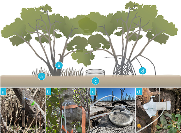
Figure 5. Diagram of ecosystem component fluxes measured via static chamber method and photographs of corresponding static chamber designs used: (a) pneumatophores, (b) mangrove stems, (c) sediments, (d) prop roots.
Download figure:
Standard image High-resolution imageAt each site, for sediment measurements, ten collars were distributed randomly around the plot. Further, a minimum of five standing stems were measured, for both living trees and snags. Stem fluxes were measured at 0, 50, and 100 cm from the base of the tree in order to test for vertical gradients in stem efflux, which can be indicative of soil rather than stem origin of stem-emitted gasses (Barba et al 2019). For red mangrove stems, an additional flux was measured at the base of a live prop root. For black mangrove stems an additional flux was measured on an adjacent pneumatophore. For each stem, a variety of ancillary data were also collected, including DBH, perimeter at each measurement height, tree stem, soil, and air temperature. Chamber incubations occurred for a minimum of 2 min for soils and 3 min for plant components.
3.1.5. Ground measurements: water chemistry
To capture water-to-air GHG exchange and its variability in mangrove waters in the Florida Everglades, a three-day spatial survey (March 2022) was conducted by navigating a houseboat from Coot Bay (25.18°N, 80.91°W), up the Joe River to the Shark River to Tarpon Bay and back while measuring pH, water temperature, salinity, CO2 and CH4 and N2O concentrations, and CO2 and CH4 stable isotopes. Surface water was pumped continuously from ∼0.5 m water depth to the on-board setup consisting of a 'showerhead' equilibrator that was connected via a closed air loop to two GHG gas analyzers, a Picarro G2201i and a Picarro G2308. (cavity ring-down spectroscopy) measuring continuous high-resolution CO2, CH4, and N2O concentrations (ppm) Surface-water conductivity (EC), dissolved oxygen (DO), temperature, pH, and colored dissolved organic matter (CDOM) were measured every minute using a calibrated multi-parameter sonde (Eureka Water Probes). Filtered sterilized discrete samples for spectrophotometric pH, dissolved inorganic carbon (DIC) and total alkalinity (Talk) were collected periodically and analyzed in the laboratory at Yale University.
3.1.6. Ground measurements: long-term carbon burial
Blue carbon stocks include the total amount of carbon buried in soil and within living and non-living biomass, both above- and below-ground, in blue carbon ecosystems (Windham-Meyers et al 2019). Long-term blue carbon burial can be estimated by multiplying the sediment accumulation rate measured from the decay of 210Pb below the surface mixed layer (usually below 30 cm depth) by the burial concentration of organic carbon (from depth profile of organic carbon). Included in this is the active uptake and preservation of CO2 within the ecosystem (referred to as carbon sequestration) as well as the long-term (>100 year; e.g. Fearnside 2002) accumulation and burial of carbon pools belowground (referred to as blue carbon storage). To better understand variability in blue carbon sequestration and storage in mangroves forests within the Everglades, we collected 1 m sediment cores using Russian peat borers that will be measured for total organic carbon (TOC) and for radioactive isotopes (210Pb for <100 year carbon sequestration and 14C for >100 year carbon burial and storage). While many studies estimate carbon stocks using carbon inventories alone (i.e. TOC), radioactive isotopes are needed to understand variability in sedimentation and will provide a better understanding of the timescales associated with blue carbon storage development in the mangrove forests.
3.1.7. Ground measurements: flux tower observations
The eddy covariance (EC) method was used to measure the exchange of trace gasses (CO2 and CH4) between wetland systems and the atmosphere throughout the Florida Everglades. Several flux towers exist in the region as part of the FCE LTER along the Shark River Slough (SRS) and Taylor Slough/Panhandle (Ts/Ph) hydrologic gradients (Malone et al, 2015). The EC towers are equipped with 3D sonic anemometers (model RS‐50, Gill Co., Lymington, England) that measure wind speed and virtual temperature, and use an open path infrared CO2/H2O gas analyzer (LI‐7500, LI‐COR, Inc., Lincoln, Nebraska), and a CH4 analyzer (LI-7700, LI‐COR Inc., Lincoln, Nebraska). Flux data are measured at 20 Hz. In addition to flux data, meteorological measurements include net radiation (CNR 1, Kipp and Zonen, Bohemia, New York) and incoming and reflected PAR (model LI‐190SB, LI‐COR, Inc., Lincoln, Nebraska), air temperature (Ta) and humidity (HMP45C, Campbell Scientific, Inc., Logan, Utah) and wind speed and direction (model 05103 RM Young, Traverse City, Michigan).
The original riverine mangrove forest tower, SRS6, was constructed in June of 2003 and the instruments were installed 27 m above the soil surface on a 30 m tower. While measurements of CO2 and H2O go back to 2004, CH4 measurements began in 2018. Air temperature is measured at 20, 15, 11, 6, and 1.5 m above the ground surface using aspirated and shielded thermometers (107 temperature probes, Campbell Scientific, Inc.). Below ground soil heat flux (HFT 3.1, Campbell Scientific, Inc.) and soil temperature (105 T, Campbell Scientific, Inc.) (Ts) are measured at 5, 10, 20, and 50 cm. Hydrologic data at this site are continuously monitored and recorded every 15 min at a station 30 m south of Shark River and 150 m west of the flux tower. Measurements included specific conductivity and temperature (600 R water quality sampling sonde, YSI Inc., Yellow Springs, Ohio) of surface well water and water level (Waterlog H‐333 shaft encoder, Design Analysis Associates, Logan, Utah). The detailed information on construction of base of tower and other supporting structure can be found in Barr et al (2010).
3.2. Airborne EC fluxes
Airborne EC (AEC) is a well-established technique for quantifying surface-atmosphere exchange of trace gasses and energy (Desjardins et al 1982). When combined with wavelet transforms (Wolfe et al 2018), AEC can characterize spatial gradients in fluxes at model-relevant scales (1–100 km). Flux footprint modeling allows for evaluation of fluxes within the context of surface properties and modeled fluxes (Hannun et al 2020, Vaughan et al 2021). Such data is complementary to ground-based observations, which integrate over a relatively small area but may better constrain site-specific processes and temporal variability.
BlueFlux AEC observations employ the NASA CArbon Atmospheric Flux Experiment payload on a Beechcraft King Air A90 flown by Dynamic Aviation and equipped with meteorological and trace gas sensors. An AIMMS-20 (Aventech) provides 10 Hz observations of 3D wind velocities, air temperature, aircraft position, and aircraft orientation (pitch/roll/yaw). This system includes a probe (mounted under the left wing) for meteorological measurements coupled with high-resolution differential GPS and inertial navigation systems. Similar systems have been utilized for airborne EC previously (Vaughan et al 2021). Ambient air is sampled through a gas inlet mounted under the right wing and transferred through a Teflon PFA tube (in the wing) to two gas sensors in the cabin. Based on analysis of cospectra, the size of flux-carrying eddies are 100–3000 m, much larger than the 15 m of space between the inlet and wind sensor. A Picarro G2401 m provides 0.5 Hz measurements of CO2, CH4, H2O, and CO, while a Picarro G2311-f provides 10 Hz measurements of CO2, CH4, and H2O. The G2401 m contains specialized pressure control systems for airborne operation and thus serves as the accuracy standard for mixing ratios, while the G2311-f provides the fast time response needed for AEC. Dry CO2 and CH4 mixing ratios are calibrated in the laboratory against NOAA World Meteorological Organization compressed gas standards with a two-point calibration.
Figure 6 maps the flight tracks from the April 2022 field campaign. Each deployment consists of 4–6 flights (25 flight hours per deployment), with five deployments planned over 2022 and 2023. The flights are designed to focus on coastal mangrove vegetation in South Florida but also include mapping over inland forests and wetlands, such as the extensive sawgrass marshes (Cladium jamaicense). The deployments are scheduled to capture seasonal and interannual variation, as well as diurnal changes, while taking into account flight safety due to weather, i.e. late-afternoon storms, hurricane season, and other flightpath restrictions. Flight duration ranges from 2.5 to 4.5 h. Typical altitude is 100 m above ground level, with occasional spirals to ascertain mixed layer depth and flux legs higher in the mixed layer (200–800 m) to determine vertical flux divergence corrections. At an altitude of 100 m and typical surface wind speeds of 5–10 m s−1, we expect 50% of the flux footprints to fall within 1000 m upwind and 90% within 5000 m. On two representative legs spanning inland forest, mangroves, and freshwater marsh, fluxes for CO2 ranged from 0 to −40 μmol CO2 m−2 s−1 and fluxes for CH4 ranged from 0 to 200 nmol CH4 m−2 s−1 (figures 7(a) and (b)). In general, the methane fluxes appear to be higher for sawgrass and CO2 uptake greater for mangroves for the April field campaign. Further flights and analysis will explore seasonal and interannual variability.

Figure 6. BlueFlux airborne operations in April 2022. White lines show tracks for airborne flux legs; note that each line may include multiple overlapping transects. White squares are long-term surface observation sites. Green patches denote Mangrove extent as of January 2022 (https://geodata.myfwc.com/datasets/myfwc::mangrove-habitat-in-florida-1/about, last accessed 21 June 2022) and the location of the SRS and TS flux towers are labeled. Inset shows the location of the operation area in Southern FL.
Download figure:
Standard image High-resolution image
Figure 7. Time series of methane (cyan) and carbon dioxide (blue) fluxes on two legs of the Everglades raster flight from 21 April 2022. The x-axis is the distance traveled over each leg, with 0 denoting the northernmost point of each leg. Maps to the right of the time series depict the flight tracks of each leg in red. Green shading shows regions of mangrove habitats. The wind during this flight was from the northeast at an average of 9 ± 2 m s−1.
Download figure:
Standard image High-resolution image3.3. Prototype carbon flux and blue carbon products
The airborne flux measurements will be used as training data for a data-driven upscaled model that will provide daily gridded CH4 and CO2 fluxes to be compared with the long-term burial rates. Given the extensive spatial and temporal coverage of the fluxes from the flights, and combined with the disaggregation of the ecosystem level fluxes to the components of water, soil and stem, and the validation with tower data, the gridded prototype products can provide the basis for a variety of studies. Figure 8 shows an example of gridded methane fluxes using training data from the seven flight days between 19th and 26th April 2022. These flights provided measurements of methane fluxes for 43 141 sample points at 500 m spatial resolution. We used the MODIS Nadir Bidirectional Reflectance Distribution Function (BRDF)-Adjusted Reflectance (NBAR, MCD43A4v006) data over the study area downloaded from Google Earth Engine. MODIS NBAR is developed daily at 500 m spatial resolution, using 16 d of Terra and Aqua data to remove view angle effects and temporally weighted to the ninth day as the best local solar noon reflectance (Schaaf et al 2002, Wang et al 2018).

Figure 8. Data-upscaling for methane using flight tracks in figure 6 to train a reflectance-based model using (a) MODIS NBAR of all seven land bands: red (620–670 nm), green (545–565 nm), blue (459–479 nm), NIR1 (841–876 nm), NIR2 (1230–1250 nm), SWIR1 (1628–1652 nm), SWIR2 (2105–2155 nm). The Everglades National Park boundary is shown in white polygons; (b) the gridded methane fluxes for April 2022; and (c) comparison between modeled fluxes from MODIS NBAR reflectance versus Terra and Aqua.
Download figure:
Standard image High-resolution image
Mean values of MODIS NBAR product between 19th and 26th April were composited per band of seven spectral bands (figure 8(a); red, NIR1, blue, green, NIR2, SWIR1, SWIR2) as model input features. The MODIS Terra land-water mask (MOD44Wv006, Carroll et al 2017) of 2015 was applied to mask open-water pixels. Sampling points from the flight lines were mapped to the MODIS grid cells by averaging FCH4 and FCO2 values of points that fell in the same MODIS pixel. This produced 1528 gridded data. An upscaling model was trained at the MODIS pixel scale using ensemble random forest regressors (Breiman 2001, Kim et al 2020). Random forest regression contains an assembly of independent trees constructed from a random subset of input data or input space (features). The generalization error converges as the forest grows to a limit, which avoids overfitting. We used the scikit-learn library in Python to build up random forest regressors with a bootstrap ensemble sampling for data. A 'tree' grew a split where a random selection of two features reduces the mean squared error (MSE) at a leaf node.
Red and near-infrared bands that have been widely used for characterizing vegetation chlorophyll, canopy structure and soil wetness were among the most important bands to model spatial variability of methane and carbon dioxide fluxes in the Everglades National Park and surrounding region. We also trained separate upscaling models on MODIS Aqua and Terra 8 day composite Level 3 surface reflectance data (MYD09A1v061 and MOD09A1v006, Vermote et al 2002, Bréon and Vermote 2012). Only pixels with good quality data were used. The RMSE of the Aqua model was 12.74 nmol m2 s−1 and 12.41 nmol m2 s−1 for Terra trained model, compared with 10.1 nmol m2 s−1 for the NBAR product. Methane fluxes mapped from NBAR data in our study area have a better spatial representation of methane emission gradients and variabilities than those from Aqua or Terra data (figure 8(c)). High methane emissions were located in inundated sawgrass marsh in the SRS and the estuarine section of Taylor Slough (figure 8(b)). Due to frequent cloud cover, the 8 day composite of Aqua or Terra data are noisier than the NBAR product over high emission marsh and low emission cypress swamp, which produced different density distributions of methane fluxes (figure 8(c)). Future work will consider how to integrate sub-daily and sub-weekly tidal and meteorological information not included in the Aqua and Terra products.
4. Anticipated results
One of the main concerns regarding 'blue carbon' as an NBS is that it considers carbon stores and long-term burial rates but overlooks non-CO2 GHG emissions that can affect (positively or negatively) the overall net radiative forcing effect of these ecosystems (Malerba et al 2022). Mangroves are intertidal ecosystems and while net autotrophic at the ecosystem scale (Duarte et al 2005, Alongi 2014), creek waters and sediments are generally a source of atmospheric CO2 and CH4 (Call et al 2015, Rosentreter et al 2018a) and can also act as a source or sink for N2O (Maher et al 2016, Reithmaier et al 2020). Along the tidal elevation gradient (creek to forest basin), mangrove coverage, species diversity, and sediment structure can change markedly, resulting in great spatial variability of GHG fluxes. The tidal systems also have large differences at diurnal time scales, which BlueFlux will address by integrating high-density timeseries from the flux towers with the more spatially expansive aircraft flux observations.
Using the upscaled methane and carbon dioxide fluxes from the NBAR-based reflectance model, we estimated for the Everglades National Park (∼6000 km2) that CO2 removals were 91 677 Mt d−1 or 33.5 Tg CO2 y−1 and CH4 emissions were 182.7 Mt d−1 or 0.06 Tg CH4 yr−1 (where Tg = teragram = 1 × 10¹² grams). To compare how much methane emissions reduces the climate mitigation potential of carbon dioxide removals, we apply the Intergovernmental Panel on Climate Change (IPCC) 100 year global warming potential of 28 and estimate that 1.7 Tg CH4-CO2-eq yr−1 are emitted to the atmosphere. This suggests that about 5% of the CO2 uptake by vegetation is offset by methane emissions. Subsequent field campaigns and modeling will integrate seasonal and inter-annual variability into these estimates as well as address and quantify the sources of uncertainty related to local and long-distance lateral fluxes and long-term carbon burial. Our upscaled estimate is similar order of magnitude to Troxler et al (2013) who also partition how much of the carbon removed from the atmosphere is transported laterally via aquatic fluxes to the Gulf of Mexico.
The BlueFlux field campaign is designed to collect detailed information on mangrove structure with multi-scale measurements of GHG fluxes. The data-upscaling approach described in section 3.3 will capture a variety of edaphic, hydrologic and disturbance gradients either through the reflectance data or through additional covariates, such as wind speed, remote-sensed forest structure using radar or lidar, and topographic information. By combining flux tower measurements that provide sub-daily time series with aircraft measurements that cover large spatial variability, the processes driving GHG fluxes can be incorporated into upscaled models. The gridded carbon flux products will provide a basis for evaluating trends over the past two decades in GHG fluxes and their spatial patterns in response to changing climate and climate extremes, hurricane history, and land management.
5. Anticipated impact
Blue carbon is integrated within many policy-guiding documents and climate mitigation policies themselves (Hilmi et al 2021). The IPCC Good Practice Guidelines for wetland inventories (IPCC 2014) and the Special Report on the Ocean and Cryosphere in a Changing Climate both discuss the consequences of maintaining and restoring these ecosystems for climate mitigation. The Blue Carbon Policy Project of the International Union for the Conservation of Nature helped guide recommendations to the United Nations Framework Convention on Climate Change's 26th Conference of Parties (COP26) in 2021. At COP26, blue carbon related goals included enhancing ambition, accelerating implementation and monitoring and verification of results.
A key aspect of NASA's CMS is to support stakeholder needs and expand partnerships with practitioners involved with climate mitigation. BlueFlux is partnered with stakeholders in (1) the private sector through the Everglades Foundation and the Environmental Leadership and Training Initiative at Yale University, (2) through federal agencies, including NASA, United States Geological Survey, the National Park Service, and National Science Foundation, (3) through tribal nations, including the Miccosukee, the Seminole Nation of Oklahoma and the Seminole Tribe of Florida, and (4) through international partnerships with the Coastal Biodiversity Resilience to increasing Extreme events in Central America. The data access policy follows NASA's Open Source Science philosophy of being freely and readily accessible, with transparent metadata and documentation.
BlueFlux intends to benefit these stakeholders by accounting for GHG exchanges from critical blue carbon ecosystems, i.e. mangroves and sawgrass marshes. The multi-source, multi-scale quality of the project also aims to allow stakeholders to access information and data from the soil, and water to the atmosphere that may support the generation and refinement of IPCC Tier 3 inventory methods, and the assessment and reduction of the uncertainties associated with current models for NGHGI (Ogle et al 2019). For example, the IPCC 2013 Supplement for wetlands currently uses a single emissions factor of 19.37 g CH4 m2 y−1 for wetland cases where salinity is <18 parts per thousand (ppt) and zero for when salinity is >18 ppt (IPCC 2014) and assumes no methane emissions for mangrove systems. Our study will help better understand how disturbance, hydroperiod and salinity gradients drive methane emissions and help provide a basis for Tier 3 approaches where relevant.
The cross-scale calibrated BlueFlux products, developed at 500–1000 m resolution for Mesoamerica and the Caribbean might also support local, and regional policies and projects on climate change adaptation and mitigation, ecosystem restoration, and carbon market. The project also provides data that can support the Global Stocktake of the Paris Agreement (GST) and the nationally determined contributions process, since it maps GHG flux time series from coastal ecosystems under varying conditions and, as consequence, highlights the history of regional carbon sinks and sources.
Acknowledgments
The BlueFlux project acknowledges core support from the NASA Carbon Monitoring System and NASA's Terrestrial Ecology Program. We would like to thank the BNP-PARIBAS foundation for their support to the CORESCAM project (Coastal and Marine biodiversity resilience to increasing extreme events in Central America and the Caribbean), from their 2019 Biodiversity and Climate Change call. We also thank the Everglades and Big Cypress National Parks and the Florida Coastal Everglades Long Term Ecological Network for their support. We thank Dr Christopher Holmes (Florida State University) for providing airborne support and Dr Brad Eyre (Southern Cross University, Australia) for providing helpful comments on an earlier draft of this manuscript.
Data availability statement
No new data were created or analysed in this study.