

Abstract
Mesoscale vortices (MVs) play an important role in balancing global atmospheric momentum, moisture, and energy, and can induce almost all types of disastrous weather. To enhance the understanding of MVs, there is a need to identify them from various types of grid data. Despite the higher detection accuracy, manual identification is gradually being replaced by numerical methods, because the former has enormous time and manpower requirements. However, after decades of research to accurately detect MVs using numerical algorithms the process remains challenging. This study proposed the use of restricted vorticity (RV) as a new metric for numerical MV identification, based on which a numerical algorithm was developed. Compared with ∼1800 manually identified MVs, the new algorithm had a hit rate of over 97%, and a Heidke skill score of above 0.9. This indicates that RV will be of great practical value, and is suitable for popularizing and applying immediately.
Export citation and abstract BibTeX RIS

Original content from this work may be used under the terms of the Creative Commons Attribution 4.0 license. Any further distribution of this work must maintain attribution to the author(s) and the title of the work, journal citation and DOI.
1. Introduction
A vortex usually refers to a flow with closed streamlines (wiki/Vortex). This type of system is one of the most common weather systems and may occur anywhere at any time (this study only focused on cyclonic vortices). According to Orianski (1975), vortices with a horizontal length scale ranging from 2 to 2000 km are referred to as mesoscale vortices (MVs). This includes mesoscale convective vortices (Davies et al 2004), southwest vortices (Ni et al 2017, Feng et al 2019), Tibetan Plateau vortices (Curio et al 2019), Dabie vortices (Zhang et al 2015, Fu et al 2017), tropical cyclones (Doyle et al 2017), extratropical cyclones (Schultz et al 2018), polar lows (Montgomery and Farrell 1992), and explosive cyclones (Allen et al 2010). MVs play an important role in the balance of global atmospheric momentum, moisture, and energy (Neu et al 2013), and they are very important to the initiation of mesoscale convective systems, when the large-scale forcing is generally weak (Song et al 2019). MVs are closely related to almost all types of disastrous weather, such as torrential rainfall (Bartels and Maddox 1991, Trier and Davis 2002), strong wind (Evans et al 2014, Grunzke et al 2017), lightning (Bovalo et al 2014, Fierro and Mansell 2018), hail (Tessendorf et al 2005, Allen et al 2020), blizzards (Zhang et al 2012, Rauber et al 2017), and dust storms (Qian et al 2002, Huang et al 2016). For this reason, MVs have long been a research hotspot in meteorology and related fields.
To investigate MVs, the first step is to identify them correctly. Manual identification is an effective method and has been widely utilized in previous studies (Menard and Fritsch 1989, Bartels and Maddox 1991, Tirer and Davis 2002, Kirk 2003, Davis and Galarneau 2009, Zhang et al 2012, Fu et al 2015, 2016, Li et al 2019, Tochimoto et al 2019). This method can guarantee a high accuracy of MV detection (Neu et al 2013, Fu et al 2016); however, with the emergence of increasing amounts of prediction/reanalysis gird data, manual identification has become inefficient because it consumes enormous amounts of time and manpower. Therefore, numerical MV identification algorithms are urgently needed. Scientists have been working to develop different algorithms since the 1990s (e.g. Murray and Simmonds 1991, Sinclair 1994, Hewson 1997, Hoskins and Hodges 2002, Zolina and Gulev 2002, Pinto et al 2005, Wernli and Schwierz 2006, Kew et al 2010, Hanley and Caballero 2012, Tuttle and Davis 2013, Hou et al 2017, Curio et al 2019, Jiang et al 2020). However, despite the great effort expended and important progresses that has been made, the detection of MVs with a high degree of accuracy is still difficult. This is because all of the identification metrics currently used in numerical MV identification algorithms have notable limitations (Hoskins and Hodges 2002, Neu et al 2013).
The metrics currently used in most numerical MV identification algorithms are: (a) sea level pressure (SLP) (e.g. Murray and Simmonds 1991, Zolina and Gulev 2002, Hanley and Caballero 2012), (b) geopotential height (e.g. Kew et al 2010, Lu et al 2017, Jiang et al 2020), (c) relative vorticity (this study only focused on the vertical component) (e.g. Sinclair 1994, Davis et al 2002, Wang et al 2011a, 2011b, Curio et al 2018), and potential vorticity (e.g. Fu et al 2015). According to the geostrophic adjustment theory (Holton 2004), for mesoscale scale systems, the pressure field adjusts to the wind field, which means that relative vorticity (calculated by the wind field) may be a more reliable metric to use for MV detection. This has been confirmed by many previous studies; for example, Hodges et al (2003) reported that relative vorticity contained more information regarding the high-frequency scale, whereas SLP and geopotential height better represent the low-frequency scale. Neu et al (2013) found that relative vorticity based algorithms would be more skillful in identifying MVs in their early stage and in detecting shallow MVs; Rudeva et al (2014) found that identification algorithms built with relative vorticity had a faster rate of identification than those using SLP/geopotential-height. However, as an identification metric, relative vorticity also has notable deficiencies because a large proportion of vorticity maxima do not represent an MV (e.g. the green plus signs in figures 1(a)–(c)), and the MV-associated vorticity maxima may be significantly displaced from the MV centroids, which are used to represent MV centers (e.g. the MVs in figures 1(a) and (b)). This will produce too many pseudovortices, which not only significantly increases the difficulty of MV identification in the next step (a numerical MV identification algorithm usually has several steps), but also reduces the final detection accuracy. Therefore, there is an urgent need to develop a more effective metric for numerical MV identification.

Figure 1. Panel (a) shows the 500 hPa geopotential height (blue solid line, units: gpm), relative vorticity (shading, units: 10−5 s−1), and stream lines (black lines with vectors) at 1900 UTC 12 April 2020. Panel (b) is the same as (a) but for 700 hPa at 1800 UTC 12 April 2020. Panel (c) is the same as (b) but for 0600 UTC 12 June 2010. Panel (d) shows the 700 hPa geopotential height (blue solid line, units: gpm), RV (shading, units: 10−5 s−1), and stream lines (black lines with vectors) at 0600 UTC 12 June 2010. The green triangle marks the minimum geopotential height, and the green '+' marks the maximum relative vorticity and RV. Panels (a) and (b) are based on ERA5 reanalysis data and panels (c) and (d) are based on CFSR reanalysis data.
Download figure:
Standard image High-resolution imageIn this study, based on the physical significance of relative vorticity, we proposed the use of a new MV identification metric, restricted vorticity (RV). Compared to relative vorticity, the use of RV does not require complicated additional processing. In most situations, RV has a much higher consistency with manually detected MVs than traditional metrics (e.g. relative vorticity, SLP, geopotential height, and potential vorticity), both in terms of MV numbers and the location of their centers (see figures 1(c) and (d)). Thus, RV provides an effective way to improve the accuracy of numerical MV identification algorithms. In addition, to the best of our knowledge, no previous studies have quantitatively evaluated a numerical MV identification algorithm. This study was based on ∼1800 manually detected MVs in China (we regarded the identifications to be true), as shown in table 1. We first compared the detection results of candidate MVs using RV (as the metric) with those using relative vorticity, geopotential height, and potential vorticity, and then we calculated two standards to quantitatively evaluate the accuracy of the RV-based numerical MV identification algorithm. For the first time, a quantitative objective evaluation of a numerical MV detection algorithm is reported here. The results highlight the effectiveness of RV as a metric for numerical MV identification. The remainder of the paper is organized as follows: section 2 presents the data; section 3 introduces the concept of RV, section 4 provides the application of an RV-based numerical MV identification algorithm and its accuracy; and finally, a conclusion is presented in section 5.
Table 1. The period and vortex numbers (number of manually detected vortexes) used for evaluation, and the corresponding hit rate and false rate of the RV-based numerical MV identification algorithm. RV = restricted vorticity, MV = mesoscale vortex, DBV = Dabie vortex, TPV = Tibetan Plateau vortex, HSS = Heidke skill score and CFSR = Climate Forecast System Reanalysis.
| Period | MV type (numbers) | Data type | Hit rate | False rate | HSS |
|---|---|---|---|---|---|
| June 2002 | DBVs (33) | CFSR (6 hourly) | 97.0% | 6.0% | 0.94 |
| July 2002 | DBVs (56) | CFSR (6 hourly) | 96.4% | 1.8% | 0.95 |
| August 2002 | DBVs (55) | CFSR (6 hourly) | 92.7% | 5.8% | 0.89 |
| June 2008 | DBVs (44) | CFSR (6 hourly) | 100% | 4.5% | 0.96 |
| July 2008 | DBVs (28) | CFSR (6 hourly) | 100% | 0.0% | 1.0 |
| August 2008 | DBVs (36) | CFSR (6 hourly) | 88.9% | 0.0% | 0.91 |
| July 2013 | DBVs (14) | CFSR (6 hourly) | 100% | 7.1% | 0.95 |
| DBV total | DBVs (266) | CFSR (6 hourly) | 95.9% | 3.4% | 0.94 |
| May 2009 | TPVs (475) | ERA5 (hourly) | 97.7% | 6.7% | 0.93 |
| July 2011 | TPVs (1045) | ERA5 (hourly) | 97.6% | 9.7% | 0.88 |
| TPV total | TPVs (1520) | ERA5 (hourly) | 97.6% | 8.8% | 0.90 |
| Both total | DBV + TPV (1786) | CFSR + ERA5 | 97.4% | 8.0% | 0.91 |
2. Data and the two types of MVs used for testing
In this study, two types of high-resolution reanalysis datasets were used for testing the performance of the RV-based numerical MV identification algorithm: (a) the hourly 0.25° × 0.25° European Centre for Medium-Range Weather Forecasts (ECMWF) ERA5 data (Hersbach et al 2020); and (b) the 6 hourly 0.5° × 0.5° National Centers for Environmental Prediction Climate Forecast System Reanalysis (CFSR) data (Saha et al 2010).
Two types of MVs in China were used to test the usefulness of RV as a metric for numerical MV identification. One was the Tibetan Plateau vortex (TPV), which is a unique type of MV that is generated over the Tibetan Plateau (Wu et al 2018). Its central level is at 500 hPa, and its typical horizontal scale is ∼500 km (Curio et al 2019). The other was the Dabie vortex (DBV), which is formed around the Dabie Mountain in the middle and lower reaches of the Yangtze River (Zhang et al 2015). Its central level is 850 hPa and its typical horizontal scale is ∼600 km (Fu et al 2016). Both TPVs and DBVs have high frequencies of occurrence, and their numerical identification is challenging. As table 1 shows, we used the 6 hourly CFSR data to manually detect DBVs, and a total of 266 DBVs (i.e. the number of times MV) was determined. In contrast, the hourly ERA5 data was used to identify TPVs manually, and a total of 1520 DBVs were identified.
To detect both types of MVs manually, we used similar standards, i.e. when a closed vortex center in the stream field coupled with a notable positive vorticity center (>1 × 10⁻⁵ s−1) appeared, and the diameter of the vortex was greater than 200 km (the lower limit of a DBV/TPV), an MV was confirmed (Fu et al 2016, Curio et al 2019).
3. Restricted vorticity
The relative vorticity is a micro concept. For a point in a fluid, it is equal to twice the point's angular velocity (the blue curved vector in figure 2(a)), whereas an MV is a macro concept, which has closed streamlines. The closed stream lines can be directly represented by the velocity circulation, which is related to the relative vorticity through Green's theorem (i.e. the surface integral of relative vorticity over a region equals the velocity circulation along its boundary line). Green's theorem guarantees that relative vorticity can be a useful metric for numerical MV identification. However, in a real situation, when calculating the relative vorticity at a point using a difference scheme (we adopted the widely used central difference scheme in this study), it is necessary to use the dots surrounding the point. This would introduce errors into the calculation. Here, we only focused on whether the surrounding dots can reproduce a consistent counter-clockwise (in the northern hemisphere) circulation (CCC) about the central point (as the vectors in figure 2(c) show).

Figure 2. Panel (a) is a schematic illustration of vorticity ζ in the horizontal grid (green lines with black and red dots), where the two black arrows show the directions and the blue solid curve with an arrow shows the rotation direction. Panel (b) shows the wind situation used to calculate the vorticity at the red dot, where the gray arrows (larger arrow means a larger wind speed) and orange arrows (only mean the wind direction) show the three wind situations in the dominant term. Panels (c)–(f) show the four typical wind situations used to calculate vorticity, where the thick orange arrows mark the wind direction of the dominant term, and the thin purple arrows mark the wind direction of the nondominant terms.
Download figure:
Standard image High-resolution imageIf the CCC condition is satisfied, the relative vorticity ζ at the central point will be positive. However, a positive ζ does not mean that the CCC condition is met. There are many situations in which the relative vorticity is positive, whereas the surrounding dots do not meet the CCC condition. This is one of the main reasons why the relative vorticity maxima may show a notable inconsistency with real MVs. Some typical examples are provided as follows. For convenience, we defined the larger terms (i.e.  and
and  ) in
) in  as the dominant terms (u and v are the zonal and meridional wind, respectively), with the remaining term being the nondominant term. The sign of ζ is only determined by the dominant term, although a total of four points are used in its calculation.
If  is the dominant term and it is positive, there are three possible situations (zero zonal-wind was not considered), as shown in figure 2(b). However, only the situation shown by the orange vectors (figure 2(b)) has the potential to satisfy the CCC condition. If the dominant term is determined as mentioned above, there are at least four situations regarding the wind direction in the nondominant terms (zero meridional-wind was not considered), as shown in figures 2(c)–(f). Of these, only the situation shown in figure 2(c) satisfies the CCC condition.
In this study, we introduced the concept of RV to ensure that: (a) the four points (black dots in figure 2(a)) used for calculating ζ at the central point (red dot in figure 2(a)) satisfied the CCC condition; and (b) the two terms in the relative vorticity have a similar relative importance, because an MV is mainly quasi-centrosymmetric. For condition (b), we defined  , which can be used to indicate the relative importance of the two terms in ζ.
4. A quantitative test
4.1. Evaluation methods
To quantitatively evaluate the accuracy of a numerical MV identification algorithm, we developed two standards. The first standard was the hit rate, which indicated of all real MVs (i.e. those that we manually detected), how many MVs are detected correctly. We set NT as the true number of MVs and NH is a number describing what proportion of the true MVs (NH ≦ NT) were correctly detected by the identification algorithm. Then, the hit rate = NH/NT, which implies that a larger hit rate means a better performance. The second standard was the false rate, which evaluated how many MVs were detected in addition to the real MVs (we considered these MVs to be false). If the identification algorithm still detected other MVs in addition to the true MVs, and the number of these false MVs is set as NF (NF ⩾ 0). Then, the false rate = NF/NT, which implies that a smaller false rate means a better performance. Following Song and Zhang (2017, 2018), we also calculate the Heidke skill score (HSS) to evaluate the identification algorithm. Its expression is as follows:
where NM = NT− NH is the number of MVs that are missed by the algorithm, and NC is the number of correct identification of no MV situations. The maximum value of HSS is 1.0, which means that the identification algorithm is perfect, and as values of HSS decrease, its performance becomes worse.
4.2. An RV-based numerical MV identification algorithm
This study developed an RV-based numerical MV identification algorithm (figure 3). Its key steps were as follows: (a) Use a 2° × 2° (the lower limit of the diameter of a DBV/TPV is ∼200 km) box to scan the 850 hPa/500 hPa RV field within the region of interest (25°N–36°N, 111°E–119°E)/(25°N–40°N, 76°E–100°E) for candidate DBV/TPV centers. The location of the center of a candidate DBV/TPV was defined as the location of the maximum RV within the 2° × 2° box. (b) Use the center of the candidate DBV/TPV to draw a box that has a side length of 2 × Rc (Rc was defined as the calculation radius). Divide the box into eight octants (figure 3) and calculate the octant-averaged winds. (c) Check how many (N is defined as the number) of the eight octants show a cyclonic rotation pattern (as shown by the octant-averaged wind in figure 3). (d) If N is above a threshold value (shown in table 2), the candidate DBV/TPV was confirmed as a qualified MV, otherwise it remained unqualified. There were three parameters (table 2) that needed to be properly determined before conducting the numerical MV identification. The values of these parameters in this study are shown in table 2.
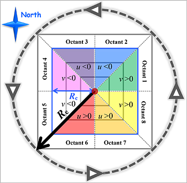
Figure 3. Schematic illustration of the eight-octant MV identification method based on RV, where the large red dot at the center represents the location of the maximum of the detected RV (i.e. the candidate MV's center), and the thick gray dashed circle with arrows shows the vortex determined by the typical effective radius (Re) of a specific type of MV (which represents the typical horizontal scale of a type of MV). The calculation radius (Rc) determined the range of grids (marked by gray and blue boxes) used for calculation, which were divided evenly into eight color shaded octants. The octant-averaged wind should satisfy the cyclonic pattern, as shown by u (zonal wind) and v (meridional wind) for the northern hemisphere situation.
Download figure:
Standard image High-resolution imageTable 2. The parameters used for detecting DBVs and TPVs, and their main information used in the detection process, where dx is the grid spacing, Rc is the calculation radius and Re is the effective radius (which represents the typical horizontal scale of a type of MV). MV = mesoscale vortex, DBV = Dabie vortex, and TPV = Tibetan Plateau vortex.
| α | Rc | N | |
|---|---|---|---|
| Objectives | Regulate the relative importance of the two terms in restricted vorticity | Determine the box which is divided evenly into eight octants | Specify the number of octants which satisfy the cyclonic rotation |
| Suggested ranges | 0.2 ⩽ α ⩽ 5 | dx < Rc < Re | 6 ⩽ N ⩽ 8 |
| DBV test (CFSR) | 0.2 ⩽ α ⩽ 5 | Rc = 2dx (0.5°) | N = 6 |
| TPV test (ERA5) | 0.2 ⩽ α ⩽ 5 | Rc = 3dx (0.25°) | N = 7 |
4.3. Quantitative evaluation results
Figure 4 shows a comparison of RV and relative vorticity, geopotential height, and potential vorticity as an MV identification metric for DBVs. Similarly to key step (a) described in section 4.2, the candidate MV centers were also determined by finding the maximum relative vorticity (figures 4(b) and (f)), minimum geopotential height (figures 4(c) and (g)), and maximum potential vorticity (figures 4(d) and (h)) within a 2° × 2° moving box. It was apparent that the use of RV (figures 4 (a) and (e)) produced a much more credible estimate of the candidate DBVs (both in terms of the number and location) than the use of the other three traditional metrics. Figure 5 shows a comparison of the use of the different metrics for detecting TPVs. Once again, the use of RV resulted in a much better performance when estimating candidate TPVs, particularly in terms of the number. Overall, compared to the use of traditional metrics, RV was found to be a much more effective metric for numerical MV identification.
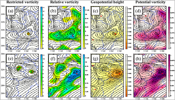
Figure 4. Panels (a) and (e) show the stream field (black line with arrows) and the RV (shading, units: 10−5 s−1). Panels (b) and (f) are the same as panel (a) but for the relative vorticity (shading, units: 10−5 s−1). Panels (c) and (g) are the same as panel (a) but for the geopotential height (shading, units: gpm), and panels (d) and (h) are the same as panel (a), but for the potential vorticity (shading, units: PVU). All panels are at 700 hPa (using CFSR (Climate Forecast System Reanalysis) data), panels (a)–(d) are at 1800 UTC 11 June 2008, panels (e)–(h) are at 1800 UTC 24 August 2008, and the red dots show the candidate DBV centers (for panels (a) and (e), they are determined by the maxima of RV; for panels (b) and (f), they are determined by the maxima of relative vorticity; for panels (c) and (g), they are determined by the minima of geopotential height; and for panels (d) and (h), they are determined by the maxima of potential vorticity).
Download figure:
Standard image High-resolution image
Figure 5. Panels (a) and (e) show the stream field (black line with arrows) and RV (shading, units: 10−5 s−1). Panels (b) and (f) are the same as panel (a) but for the relative vorticity (shading, units: 10−5 s−1). Panels (c and g) are the same as panel (a) but for the geopotential height (shading, units: gpm). Panels (d) and (h) are the same as panel (a), but for the potential vorticity (shading, units: PVU). All panels are at 500 hPa (using ERA5 data), panels (a)–(d) are at 1800 UTC 11 June 2008, and the black crosses show the candidate TBV centers.
Download figure:
Standard image High-resolution image
Based on the numerical MV identification algorithm suggested in section 4.2, we conducted MV detections for 266 DBVs that were manually confirmed in a 7 month period (table 1). The hit rate ranged from 88.9% to 100%, with a mean value of 95.9%. The false rate ranged from 0% to 7.1%, with a mean value of 3.4%. The HSS ranged from 0.89 to 1.0, with a mean value of 0.94. For TPVs, we focused on 1520 manually detected vortices (table 1) that were confirmed in a 2 month period. The hit rate was above 97%, the false rate was below 10%, and the HSS had a mean value of 0.90. Overall, for both types of MV, the average hit rate was ∼97.4%, the average false rate was ∼8.0%, and the average HSS was ∼0.91. In contrast, for the traditional numerical MV identification algorithms based on relative vorticity (Curio et al 2018), geopotential height (Jiang et al 2020) and potential vorticity, the highest average hit rate (of the three algorithms) was ∼81.6%, the lowest average false rate was ∼15.1%, and the largest average HSS was ∼0.76 (not shown). This indicates that the RV-based numerical MV identification algorithm shows a much better performance than the traditional algorithms, and therefore is of great practical value.
The horizontal resolution of the data used for numerical MV identification tends to affect the detection accuracy. On the one hand, a higher resolution contributes to both a reduction in the miss rate of candidate MVs in step (a) (section 4.2) and to obtain higher-resolution octant-averaged winds in step (b), both of which lead to improvements in the hit rate. However, on the other hand, the identification of more candidate MVs provides more opportunities to make false MV detections. Therefore, as the horizontal resolution becomes higher, the hit rate and false rate both tend to increase (table 1), with the false rate grows rapider than the hit rate. This results in an overall decrease in HSS (table 1), which means that the performance of the numerical MV identification algorithm becomes worse.
5. Conclusion and discussion
Due to their important role in balancing global atmospheric momentum, moisture, and energy, and their close relationship with almost all types of disastrous weather, MVs have long been a research focus. The accurate detection of MVs is of critical importance in MV studies. With the emergence of increasing amounts of grid data, numerical identification algorithms have become a much more efficient way of detecting MVs than manual identification. However, after decades of research, the development of an accurate numerical MV identification algorithm still remains a very challenging task. One of the main reasons for this is that all of the metrics used for MV detection have notable limitations. Most of the algorithms currently in use need a metric to determine MV candidates, based on which further checks are made to confirm the final qualified MVs. A better metric could lower the miss rate of valid MV candidates (those MV candidates that can finally be confirmed as real MVs are classed as valid MV candidates, otherwise they are invalid MV candidates) and reduce the number of invalid MV candidates, both of which will improve the final MV detection accuracy.
In terms of physical significance, this study proposed the use of a new metric for numerical MV detection, RV, which does not need any complicated additional processing. This metric resulted in a much better performance than the application of other widely used metrics, both in the representation of MV numbers and the location of their centers. Based on this metric, we proposed a numerical MV identification algorithm, and quantitatively evaluated its accuracy in detecting two types of MVs in China. It was found that, on average, the algorithm had a hit rate of more than 97%, a false rate of less than 10%, and an HSS of above 0.9. This indicated that the RV-based numerical MV identification algorithm will be of great practical value. However, in this study, we only tested the effectiveness of the RV as an MV identification metric in one algorithm, and the test was merely conducted on two types of MVs based on two types of reanalysis data. This will have limitations to comprehensively evaluate the real practicability of the RV. In the future, different types of MVs and a larger number of MVs will be used to further check the effectiveness of the numerical identification algorithm developed in this study. We will also test more combinations of the three parameters shown in table 2, which will improve the performance of the algorithm. The relationship between a dataset's horizontal resolution and the accuracy of a numerical MV identification algorithm will be further investigated. In addition, because it is effective and easy to calculate, we strongly suggest that practitioners should use RV as a metric for determining MV candidates in their numerical MV identification algorithms.
Acknowledgments
This research was supported by the National Key R&D Program of China (Grant No. 2019YFC1510400), the National Natural Science Foundation of China (Grant Nos. 41775046, 42075002, 91637211 and 41861144015), and the Youth Innovation Promotion Association, Chinese Academy of Sciences.
Data availability statement
The data that support the findings of this study are openly available at the following URL/DOI: www.ecmwf.int/en/forecasts/datasets/reanalysis-datasets/era5.