

Abstract
Impact-based, seasonal mapping of compound hazards is proposed. It is pragmatic, identifies phenomena to drive the research agenda, produces outputs relevant to stakeholders, and could be applied to many hazards globally. Illustratively, flooding and wind damage can co-occur, worsening their joint impact, yet where wet and windy seasons combine has not yet been systematically mapped. Here, seasonal impact-based proxies for wintertime flooding and extreme wind are used to map, at 1° × 1° resolution, the association between these hazards across Europe within 600 years as realized in seasonal hindcast data. Paired areas of enhanced-suppressed correlation are identified (Scotland, Norway), and are shown to be created by orographically-enhanced rainfall (or shelter) from prevailing westerly storms. As the hazard metrics used are calibrated to losses, the maps are indicative of the potential for damage.
Export citation and abstract BibTeX RIS

Original content from this work may be used under the terms of the Creative Commons Attribution 4.0 license. Any further distribution of this work must maintain attribution to the author(s) and the title of the work, journal citation and DOI.
1. Introduction
Considering hazards in isolation may both over- and under-estimate risk [1–4], and 'compound risk' is emerging as a term to encompass research to identify and understand the impact of combined hazards [5]. Over meteorological timescales (hours to weeks), even the joint behaviours of hazards whose origin involves notably different physical processes (e.g. damaging wind, extreme cold or heat, fluvial flooding, storm surge) is widely studied [6–12]. Over climatological timescales (seasonal to annual), often invoking a climate mode such as the North Atlantic Oscillation (NAO), there are multi-hazard reviews [13], but a focus has been on individual hazards [14–17] or pairwise extremes of a single variable such as temperature (hot/cold) or precipitation (wet/dry) [18, 19]. Links between potentially time-lagged events of different hazard types via persistent underlying environmental conditions [2, 20] are less studied, especially when also adopting an impact-centric approach. Using the hazards of flooding and extreme wind in Europe as an example, we illustrate that impact-based mapping can identify scientifically interesting phenomena whilst using metrics (proxies) related to aggregated risk over a planning timescale that are of interest to infrastructure operators, government agencies, and (re)insurance.
Inland flooding and extreme wind are two of Europe's most impactful hazards [21]. They are commonly assessed separately [14, 22, 23] although, at meteorological timescales, case studies of strong storms (low-pressure systems, extratropical cyclones) show both classes of damage can co-occur during the same weather system [24–28]. Intriguingly, when only short timescales (<72 h) are used to map correlation in the extremes of precipitation and wind across Europe [12], the dependency is weak in Great Britain (GB). In contrast, a substantive correlation for the GB is proposed to exist ( 0.4–0.7, p< 0.05) in longer time windows of weeks up to a year [2, 4, 11, 29]. A way to reconcile these observations is the proposal of Hillier et al [2] that compound risk is elevated by a systematic, multi-storm relationship on timescales up to seasonal (hours to months), driven by persistent underlying environmental conditions. It has not yet been possible to fully assess this idea as the GB estimates represent a single national figure [2, 11], short time-series of about 15 years [2, 4], or are from climatic variables that are not established to be metrics relating to impact (e.g. [29, 30]). Thus, to overcome these limitations, we advocate using seasonal-scale and impact-based proxies for hazard to map where flooding and extreme winds do or do not compound across Europe.
2. Method & data
2.1. Selection of metrics for correlation
In the context of natural hazards, risk is the possibility of an adverse consequence, so investigations of compound risk select proxies for impact [2, 29, 31, 32]. Types of potentially useful impact proxy can be distinguished by how directly they relate to experienced impacts, and by the timeframe they represent (figure 1). Here, the hypothesis is that the hazards of flooding and extreme wind are linked by persistent underlying environmental conditions [2, 4], so hazard metrics at a seasonal (climatic) timescale are selected as proxies for impact (figure 1—blue box with a dashed outline). Over a season stochastic, sporadically occurring and relatively uncommon extremes accumulate, permitting any coherent 'signal' of correlation to be detected most readily. By using this timeframe, any sub-seasonal time-lags between events are implicitly accounted for; lags of up to 14 days are known and thought to arise from storm sequences [11], but other time spans and physical mechanisms may also exist.
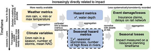
Figure 1. Two-dimensional typology of proxies for the impact of natural hazards. On the x-axis, variation is in how directly proxies are related to impact, ranging from meteorological (weather/climate) variables to quantifications of particular classes of damage such as insurance losses. Proxies may cover short or long durations, depicted on the y-axis. The blue box with a dashed outline highlights the seasonal-scale, impact-based hazard metrics that are advocated here as useful proxies for work on compound hazards.
Download figure:
Standard image High-resolution imageIn the typology of figure 1 hazard metrics are proxies for impact, which are based on weather/climate metrics; without risk of an impact, there is no hazard. There may be intermediate modelling (e.g. hydrological, hydraulic) but the crucial factor is that the metric, such as flood water depth, can be linked to eventual impact. This study uses hazard metrics derived by explicit and quantitative calibration to loss data. This approach avoids the limitations typically associated with loss data (spatially sparse, short term) whilst being 'impact-based' in that the metrics are designed to directly relate to the potential for loss should an asset exist in an affected location (e.g. [33]). Our hazard metric for extreme wind is based on regressions against loss data in previous studies, whilst a surrogate measure for flood hazard is proposed based on a calibration to losses conducted within this paper. Both metrics are outlined and justified below.
The seasonally aggregated, impact-based hazard metric used in this study for extreme wind is  , with
  for
for . In this relationship
  is daily maximum 10 m gust wind speed, c is a threshold over which damage is thought to occur, and the summation is across a season of data. Whilst a percentile might be used to define the threshold c [34], a value of 20 ms−1 is taken because damage to buildings increases markedly and non-linearly above this [35, 36]. v3 is used to account for this non-linearity as total power dissipation in wind storms, the energy available to do damage, rises roughly as v3 [15, 33, 37, 38]. Thus
  , is a well-established hazard metric, taken here as an aggregate over a season, which is designed and calibrated to linearly relate to the potential for wind damage and is thus a proxy for impact. Sensitivity tests for the choice of c are in Supp. Mat. section SM2.
The seasonally aggregated, impact-based hazard metric used in this study for flooding is  , with
  where R is total daily precipitation in mm and the summation is across a season. Aggregated winter precipitation is a common climatic variable, but is proposed as a hazard metric, a surrogate for the hazard of flooding, on a two-fold basis. First, antecedence (e.g. via soil saturation) is important for precipitation-driven hazards including flooding [11, 39, 40], and so integrating rainfall preceding events into a metric is likely beneficial. Secondly, HR observations in the period 2006–2019 correlate with losses from delays on the rail network of Great Britain (GB), an empirical demonstration that HR has some descriptive power with respect to damage. See Supp. Mat. section SM1 for the analysis underpinning this assertion of correlation (
 = 0.63, p = 0.0012, figure S1 (available online at https://stacks.iop.org/ERL/15/114013/mmedia)), which also contains sensitivity tests for the functional form of HR. In the typology of figure 1, therefore, summed precipitation (
 ) is a climate metric, but is also a hazard metric directly related to the potential for damage by flooding. This last property of
  helps in producing outputs of relevance to stakeholders (section 5).
2.2. Data
 and R data are from SEAS5, the ECMWF Seasonal forecast System 5, re-gridded to 1° × 1° [41, 42]. Each member of the SEAS ensemble (versions 4 or 5) is a physically consistent realisation of a potential reality [43, 44]. SEAS5 hindcasts have 25 members spanning 24 years (1993–2016) considered by ECMWF to be most relevant to the current day in the context of climate change [45]. Simulations run for 7 months, and September re-forecasts are chosen to capture the 'winter' half-year (Oct–Mar) when it is assumed the imprint of initialization conditions will have faded and the ensemble diverged sufficiently [44]. Namely, September itself is excluded to remove 'real' weather. This approach [43, 44, 46–49], as used here, gives 600 simulated years (24 years × 25 members) that might plausibly have occurred.
2.3. Mapping method
Compounding is mapped (figure 2(e)) by an increase (U) in mean wind hazard ( ) in the wettest one third as opposed to the driest one third of years; namely, a composite analysis (e.g. [16, 24, 50]) where a fraction (f = 0.333) of years are taken as wet. The statistical significance of U is determined by a t-test. Correlations, Pearson's (rp) and Spearman's rank (rs), between
  and
and  are examined at selected sites to support this mapping (figures 2(a–d) and S2). To help understand the potential effects of compounding upon impact, exceedance probability (EP) curves are plotted to contrast the wet and dry states (figures 2(h–j)). For these conditional probability distributions, the statistical significance of the difference between states at each return period is determined by a stochastic simulation (10 000 iterations), which determines if differences from an uncorrelated state exist [2, 51–53]. The procedure to calculate aggregate exceedance probability (AEP) curves is standard [21], and the use of conditional probability distributions is placed in the context of other widely used approaches in a review by Hao et al [54]. Whilst noting advances in statistical modelling multivariate extremes [6, 53–57], to make implementation of the approach as pragmatic as possible by academics and practitioners, we have selected the simplest sufficient methods.

Figure 2. Impact-based estimate of compounding between the hazards of flooding and extreme wind. (a)–(d) Scatter plots of the seasonal hazard metrics  and
and  , with ordinary least squares best-fit lines and 3
 confidence intervals, at sites W/E/C/N located in panel (e). (e) Map of increase in hazard (U) in wet over dry years, with f = 0.33.
  . Circles indicate a lack of statistical significance. (f) Orientation of winds on windy (>99th percentile) days for sites W and E, which is consistent with weather station data [58]. (g) as panel (f) but for wet days. (h)–(j) AEP curves for
  , for wet (blue) and dry (red) seasons at the three sites. Differences given at 10 and 40 year return periods. Where statistically significant, p values are in []; *<0.1, **<0.05, ***<0.01. Site locations: W (−006°, 56°), E (−002°,56°), C (−002°, 52°), N(001°, 61°).
Download figure:
Standard image High-resolution image3. Results: impact-based map of compounding hazards
To build upon the existing studies of Great Britain (GB) [2, 4, 11, 29], and previous mapping that used short time windows (24–72 h) [12], impact-based metrics for flooding ( ) and extreme wind (
 ) are used to map how these hazards compound across Europe on a seasonal timescale (figure 2(e)). In the Atlantic to the north and west of GB, there is an increase of roughly +100% in hazard related to extreme wind during wet years (pink). If this is taken as a background level of correlation, similar to Central site C (figure 2(c)), it is modified across the north of GB; compounding is enhanced to the west (Western site W, figure 2(a)) and suppressed to the east (Eastern site E, figure 2(b)). Similar patterns of enhanced-suppressed correlation occur across Scandinavia (Norway/Sweden) and the Iberian Peninsula. Elsewhere, the background level of positive correlation (∼100%) is present across northwest and central Europe (France, Germany), whilst compounding is low in magnitude and statistically insignificant (white/blue colours, circles) over a broad region in the south and east of Europe (e.g. Italy). This spatial pattern (relative magnitudes) of compounding in figure 2(e) is broadly insensitive to the measure of correlation used in the mapping (U, rp, rs), threshold c (fixed value or percentile), fraction f of years defined as 'wet' or 'dry', or indeed a shorter Nov–Feb winter (figure S2); see Supp. Mat. section SM2 for detail of the sensitivity tests.
In terms of wider implications, figure 2 demonstrates that using impact-based seasonal hazard metrics is a pragmatic means of mapping compounding hazards; the data are global and readily available, the metrics are easy to compute, and statistical tests basic. In detail, we acknowledge that local (sub-grid) associations and variations are not captured, perhaps on exposed hilltops outside mountainous areas (e.g. SW England) or between neighbouring valleys [59], and that some mechanisms for flooding such as snow melt (e.g. [40]) are not accounted for.
4. Discussion: enhanced compounding and correlation shadows
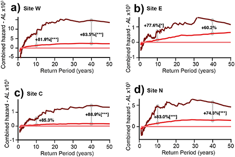
Figure 2(e) presents a view of the potential for the hazards of flooding and extreme wind to combine at seasonal timescales. There are both similarities to, and differences from, the only such prior mapping work, which considered co-occurrence within short (≤72 h) timeframes [12]. The areas of strongest short-term correlation were in North and Baltic Seas [12]. These are muted in figure 2(e), leaving paired areas of enhanced-supressed risk more distinct (Norway, Iberia, GB, South Sweden, South Italy). Given that the data used in the two studies were similar (ECMWF, 1° × 1°), why are certain patterns evident with increased clarity in figure 2? Statistical simulation modelling (detailed in Supp. Mat. section SM5) provides an explanation (figure 3). At sites in figure 2 where compounding is significant (W/C/N), figure 3 shows that the majority (∼70%–90%) of the compounding effect upon combined hazard is plausibly attributable to a relationship between the hazards at timescales over 72 h. Thus, without being in conflict with observations that flooding and wind hazards combine within individual storms [12, 24–28], figures 2 and 3 support the proposal [2, 4, 11, 29] that persistent underlying environmental conditions might enhance compounding of the flood-wind hazard by acting across multiple storms. A striking difference between figure 2(e) and mapping of short-term correlation [12] is in the region of GB. We therefore choose this area to investigate the patterns and mechanisms at work in more depth and detail, firstly where correlation is enhanced in the north-west, and then where it is suppressed in the north-east.
Figure 3. Breakdown of timescales contributing to compounding at the four sites. All panels are Aggregate Exceedance Probability (AEP) plots. AL is an estimate of combined hazard for flooding and extreme wind. AL is displayed as a difference from a simulated condition of independence between the hazards (pink line, condition C). Data directly from SEAS5 (dark red, condition A) plot above a condition in which associations between extremes within a 72 h window are retained but any longer-term relationships (e.g. monthly) are removed (red, condition B). Numerical differences between conditions A and B, due to longer term (from 72 h up to seasonal) effects, are shown at 10 and 40 years return periods (vertical grey lines). Where statistically significant, p values are in []; *<0.1, **<0.05, ***<0.01. Total (and average) of AL is identical in all 3 conditions, merely re-distributed.
Download figure:
Standard image High-resolution image
Flooding and wind hazard metrics in Great Britain compound most strongly in the north, to the west of the hills that run northwards from the Pennines into the Scottish Highlands (figure 2(e)). Storms and strong winds predominantly hit GB from the south-west (figure 2(f)) [14, 24, 58]. In these low-pressure frontal systems, the heaviest topographically enhanced rainfall occurs in the warm sector of the depressions in association with strong winds there [60–62]. This orographic enhancement over moderate amplitude topography is widely thought to be caused by the seeder–feeder mechanism [62–64], and the resulting rainfall is the main driver of flooding in affected areas (e.g. [65–67]). In SEAS5, these behaviours are evident in the agreement of wind directions for the windiest and wettest days at Site W (figures 2(f–g), blue), and in the high correlation between wind and rain ( and R) at site W both in daily data (Supp. Mat. section SM3,
  = 0.607, p < 0.01) and the seasonal hazard metrics (figure 2(a)). So, the enhancement of joint flood and wind hazard in the north-west of GB is compatible with a well-established understanding of physical processes acting there. Furthermore, the expected behaviours are evident in the SEAS5 data, suggesting that it is appropriate to interpret other patterns that emerge from the SEAS5 data. Thus, the existing understanding is demonstrably not a complete explanation because the very windiest days at site W are wet but not the wettest ones (figure S3); see Supp. Mat. section SM3 for details. Namely, storms impacting site W either tend to be wet or windy, not extreme in both. Why? We suggest that this is because storms with the most damaging winds are likely to still be actively interacting with the jet stream, but those with the most extreme rain are probably not. Such interaction is known to intensify storms, increasing
  and wind damage potential, whilst simultaneously causing them to travel rapidly [68, 69]. This would allow storms with the most intense winds less time than slower-moving systems to rain at any given site on the ground. The translational speed of extratropical storms impacting Europe adds only a minor amount to
  [21, 70], so this is probably not a major factor. This conceptual model is based on an established physical mechanism, and is an explanation for why persistence (i.e. >72 h) appears to play a role in creating the enhanced correlations in figures 2 and 3. It is not possible yet, however, to fully answer the question posed at the start of this paper and say whether the correlation mainly arises from the clustering of storms within the relatively short time windows (
 14 days) that create widespread flooding [11, 23, 71] or from persistence on climatological timescales (up to months) to create wet and stormy winters [4, 29, 32, 72–74].
East of the hills, correlation is suppressed, to which we give the label 'correlation shadow' (figures 2(b) and (e)). As a potential contributor to such features Martius et al [12] invoked the Föhn effect to generate a rain shadow, but did not discuss detail or physical mechanisms [75–78]. Most simply, the decorrelation arises because winds bearing the most intense rain to site E (northerly) come from a different direction to the strongest winds, which are from the south-west and not the north (figures 2(f–g), Supp. Mat. SM3). Why does this arise? Daily  values show that the strength of the severest gusts within a 24 h window at sites E and W is strongly related (
 = 0.773, p < 0.01), indicating that both typically arise from the same weather patterns, but extreme rain does not commonly follow at site E (
 = 0.069); see Supp. Mat. section SM3 for details. So, the key to understanding figure 2(e) is the difference in site-specific response to a similar set (figure S4) of impacting weather patterns or air masses. The concept of a rain-shadow [12, 75, 76] cannot be as readily invoked in GB as it is for larger mountains [77, 79]. However, the strongest rain-shadow effect in the type of low pressure frontal systems that impact GB occurs for precipitation in their warm sector of [62, 77, 80, 81], which is exactly the situation driving the compounding effect at site W (see above). That is, it is possible to propose that enhanced orographic precipitation on the windward western side of the topography partially dries the air mass, reducing rainfall in the lee. Thus, the correlation shadow can be partially understood as a consequence of the seeder–feeder mechanism [62], potentially reinforced by tendencies towards mutual exclusivity between wind directions within a season. At a seasonal level, the wind directions (weather types) related to flood hazard and extreme wind at site E are known to trade-off with each other [82–84]. In particular, when westerly winds are common those from the north and east occur less frequently (figure S5). This effect might in theory induce inverse relationships [4], but does not appear to be strong enough to do so as none of the negative correlations in the mapping are statistically significant (figures 2(e) and (i)).
In summary, this example involving the hazards of flooding and extreme wind in GB highlights that using seasonal impact-based hazard metrics can identify phenomena to investigate further (e.g. with daily data) and poses questions to drive future research. How does the mechanism driving GB's correlation shadow compare to that of Scandinavia or the western USA? How prevalent is each type of extra-tropical correlation shadow globally? How strong is compounding in the most extreme seasons and rarest events? How will these change in future?
5. Impact of compounding effects
Many stakeholders, such as the (re)insurance sector or a rail network provider, need to understand rare and extreme years for the purposes of planning. Will the compound aggregate loss in a season likely exceed their limits permitted by regulation, repair capacity or financial reserves? A correlation driven by moderately extreme but frequent environmental conditions is likely not a concern, whereas a dependency that exhibits itself as both very severe flooding and wind damage in the same year would be. In this context, securely establishing (p< 0.05) that wind hazard (HW) is elevated in wet years out to return periods up to ∼50 years (figures 2(h) and (j)) is an important result for GB. With wet years explicitly linked (calibrated) to increased flooding impacts (figure S1), and strong evidence that HW reflects wind damage (section2.1), this lends weight to the idea that the flood-wind correlation identified for both hazard and risk from relatively short time series in previous studies [2, 4, 11, 12, 29] is also present at higher return periods. This inference about rarer, more extreme co-occurrences is only possible as the hazard proxies (HR, HW) draw upon 600 years of SEAS5 data, and is lent significant additional weight in terms of practical interpretation as both hazard metrics are impact-based in that they have been calibrated to the observed impacts (section 2.1). As such, results from the analysis of hazard are indicative of the potential for damage in both the AEP curves (figures 2(h–j)) and the mapping (figure 2(e)). In short, the use of seasonal, impact-based hazard metrics has allowed us to build additional understanding of real-world relevance over and above that possible from the relatively short observational record.
6. Conclusions
By applying seasonal, impact-based hazard proxies to map how flooding and extreme wind compound across Europe, using SEAS5 data, our view is that such mapping is useful for three main reasons:
- 1.It is a pragmatic, self-consistent (i.e. using similar data) means to map compounding hazards across large regions using publicly available data (e.g. SEAS5). This said, where possible we advocate site-specific studies using alternative data (e.g. river flows, weather station data) and higher resolutions (spatial and temporal) to validate the observations and gain deeper process-based understanding (e.g. [85]).
- 2.The mapping identifies phenomena (e.g. correlation shadows) to drive the research agenda, posing questions and generating hypotheses about atmospheric behaviour for future investigation and testing.
- 3.The outputs (e.g. % increase in losses, AEP curves) are seasonal, at a time-scale relevant to many stakeholder's resource planning horizons, and thus of direct real-world relevance.
This approach could readily be applied to different regions, or to diverse and potentially time-lagged hazard combinations (e.g. landslide, snow, heat, wind).
Acknowledgments
We thank Rob Wilby and Alex Alabaster for their comments on early drafts of this manuscript, and two anonymous reviewers for their constructive critique of the submitted version. Both of these improved the paper. Hillier is funded by the UKRI, NERC KE Fellowship NE/R003297/1.
Data availability statement
The data that support the findings of this study are openly available at the following URL/DOI: https://cds.climate.copernicus.eu/#!/home.
Author contributions
Dixon conceived the work. Hillier and Dixon together devised and conducted the analyses, reviewed existing literature, discussed the results and wrote the paper.