


Abstract
Arctic landscapes are changing rapidly in response to warming, but future predictions are hindered by difficulties in scaling ecological relationships from plots to biomes. Unmanned aerial systems (hereafter 'drones') are increasingly used to observe Arctic ecosystems over broader extents than can be measured using ground-based approaches and are facilitating the interpretation of coarse-grained remotely sensed data. However, more information is needed about how drone-acquired remote sensing observations correspond with ecosystem attributes such as aboveground biomass. Working across a willow shrub-dominated alluvial fan at a focal study site in the Canadian Arctic, we conducted peak growing season drone surveys with an RGB camera and a multispectral multi-camera array. We derived photogrammetric reconstructions of canopy height and normalised difference vegetation index (NDVI) maps along with in situ point-intercept measurements and aboveground vascular biomass harvests from 36, 0.25 m2 plots. We found high correspondence between canopy height measured using in situ point-intercept methods compared to drone-photogrammetry (concordance correlation coefficient = 0.808), although the photogrammetry heights were positively biased by 0.14 m relative to point-intercept heights. Canopy height was strongly and linearly related to aboveground biomass, with similar coefficients of determination for point-intercept (R2 = 0.92) and drone-based methods (R2 = 0.90). NDVI was positively related to aboveground biomass, phytomass and leaf biomass. However, NDVI only explained a small proportion of the variance in biomass (R2 between 0.14 and 0.23 for logged total biomass) and we found moss cover influenced the NDVI-phytomass relationship. Vascular plant biomass is challenging to infer from drone-derived NDVI, particularly in ecosystems where bryophytes cover a large proportion of the land surface. Our findings suggest caution with broadly attributing change in fine-grained NDVI to biomass differences across biologically and topographically complex tundra landscapes. By comparing structural, spectral and on-the-ground ecological measurements, we can improve understanding of tundra vegetation change as inferred from remote sensing.
Export citation and abstract BibTeX RIS

Original content from this work may be used under the terms of the Creative Commons Attribution 4.0 license. Any further distribution of this work must maintain attribution to the author(s) and the title of the work, journal citation and DOI.
1. Introduction
Arctic ecosystems are warming rapidly (IPCC 2013) and plant communities are responding (Myers-Smith et al 2011, Elmendorf et al 2012, 2015, Myers‐Smith et al 2019). Shrub growth is climate sensitive (Elmendorf et al 2012, Myers-Smith et al 2020) and increases in shrub abundance and decreases in bare ground in plant communities have been reported at sites around the tundra biome (Myers-Smith et al 2011, Elmendorf et al 2012). However, there is limited understanding of the controls on vegetation change in tundra plant communities (Post et al 2019, Myers-Smith et al 2020). We do not yet have standardised methods of quantifying changes in tundra plant canopy structures and growth across the landscape and there are few allometric relationships relating observable plant dimensions to aboveground biomass in Arctic ecosystems (Berner et al 2015). One of the key challenges in tundra ecological monitoring is acquiring scale-appropriate observations due to the small growth forms of many plants in this large extent and often less accessible biome (Fisher et al 2018).
Remote-sensing approaches have been widely employed to gather information about changing Arctic landscapes (Walker et al 2003, Jia et al 2009, Berner et al 2015, Bartsch et al 2020, Myers-Smith et al 2020). In tundra ecosystems, there is a critical scale gap between biome-wide coarse-grain observations from satellite-based remote sensing (with pixels typically measuring between 64 km2 and 100 m2) and in situ observations collected at fi-ne spatial scales typically over a few meters (Santin-Janin et al 2009, Riihimäki et al 2019, Bartsch et al 2020, Myers-Smith et al 2020). Bridging this scale gap requires the integration of observations at intermediate scales. Unmanned aerial systems (hereafter 'drones') are one possible platform for deploying sensors to collect fine-resolution data at landscape scales (Anderson 2016), which have now become widely used for collecting environmental data (Assmann et al 2018, Assmann et al 2020, Howell et al 2020, Karl et al 2020). However, empirical work is needed to relate remotely-sensed attributes to ecological variables and inform scientific interpretations (Räsänen et al 2019).
Fine-scale measurements of three-dimensional plant structure can inform biomass prediction (Greaves et al 2015, 2017, Cunliffe et al 2016, Fraser et al 2016, Poley and Mcdermid 2020). Such methods have been demonstrated with ground-based and airborne light detection and ranging (LiDAR) observations in Arctic tundra landscapes (Greaves et al 2015, 2017), but also with aerial photogrammetry surveys leveraging advances in computer vision approaches (Fraser et al 2016, 2019, Alonzo et al 2020). However, few studies have tested the correspondence between photogrammetrically-determined canopy height and in situ measurements Arctic plants. Such testing is necessary to inform the successful integration of drone-derived products into existing ecological monitoring programmes in the tundra biome.
Spectral reflectance measurements from optical remote sensing have long been used for vegetation studies (Jia et al 2003, Walker et al 2003, Myers-Smith et al 2020). Spectral reflectance data can be used to calculate vegetation indices such as the normalised difference vegetation index (NDVI), which contrasts the reflectance in the red portion of the spectrum that is maximally absorbed by chlorophyll with the near-infrared (NIR) portion that is highly reflected by leaf and canopy structures (Buchhorn et al 2016). Several studies have shown that NDVI can be good predictor of photosynthetic tissue biomass (here after phytomass) in Arctic ecosystems (Boelman et al 2003, Walker et al 2003, Hogrefe et al 2017), and NDVI has often also been considered a predictor of total aboveground biomass (Berner et al 2018, Myers-Smith et al 2020). However, different plant tissues have different reflectance properties (Bratsch et al 2017, Räsänen et al 2019), and aboveground biomass is dominated by non-photosynthetic tissues, such as woody stems, in many vegetation communities such as shrublands (Epstein et al 2012). Logistical challenges have limited the number of empirical studies that have been able to test the relationship between NDVI and total aboveground biomass (Berner et al 2018; although see Boelman et al 2003, Goswami et al 2015). Furthermore, there is commonly a scale mismatch between the extent sampled for spectral reflectance (i.e. the ground sampling distance of a remotely-sensed pixel) and the extent over which aboveground biomass is quantified (Berner et al 2018, Karlsen et al 2018). The capacity of peak NDVI to explain variation in total biomass requires further evaluation given the widespread consideration of NDVI as a predictor of total aboveground biomass, combined with the increasing accessibility of spectral reflectance data at ever-finer spatial resolutions (Fraser et al 2017, Berner et al 2018, Riihimäki et al 2019, Assmann et al 2020).
In this study, we conducted spatially explicit-comparisons between ground-based and drone-based measurements of canopy height, NDVI and biomass to address biomass monitoring in tundra ecosystems. We worked across a Salix richardsonii to graminoid ecotone on a shrub-dominated alluvial fan at a focal tundra research site on Qikiqtaruk–Herschel Island. We examined whether drone data collection combined with image-based modelling approaches yielded high-fidelity measurements of vegetation attributes. We tested the correspondence among (i) canopy height models derived from aerial photogrammetry and in situ point-intercept methods, (ii) canopy height and aboveground biomass of vascular plants, and (iii) NDVI values obtained at different spatial grains and total vascular plant biomass, photosynthetic biomass and leaf biomass. Our analyses tested the extent to which drone-based methods can be used to monitor vegetation canopies to infer tundra biomass and productivity.
2. Methods
2.1. Site description
We conducted our study on Qikiqtaruk–Herschel Island in the Canadian Arctic. Tundra vegetation communities here range from graminoid- to shrub-dominated and are underlain by organic soils and ice-rich permafrost. This site has undergone marked ecological changes in community composition, increases in canopy height and vegetation abundance, decreases in bare ground, and an advance in leaf emergence and flowering over nearly two decades of ecological monitoring (Myers‐Smith et al 2019).
2.2. Field sampling
Our study area encompassed a graminoid-shrub ecotone at the edge of a wet willow shrub-dominated alluvial fan (69.571°N, 138.893°W) (figure 1). We established two adjacent sites, a 0.5 ha area to the north was allocated for monitoring canopy structure and biomass change over time (coordinates in table S4), and an adjacent sampling area to the south contained the harvest plots for calibrating allometric relationships between height or NDVI and biomass. Both the monitoring and harvesting areas were selected to be representative of the full distribution of canopy heights that we observed in the field (see figure S8 for comparison of value distributions) (available online at stacks.iop.org/ERL/15/125004/mmedia).

Figure 1. Overview of the study site encompassing a graminoid-shrub ecotone. The panels indicate: location of Qikiqtaruk–Herschel Island in the Western Canadian Arctic (a), location of the study site on an alluvial fan to the east of the Island at 69.571°N, 138.893°W (b), an aerial oblique photograph of the graminoid to shrub ecotone, looking southwest (c), and true colour orthomosaic at 4 mm spatial resolution (d). The orange flags (in c) indicate some of the 36 harvest plots (blue squares in d) and the white squares (in c) indicate some of the 26 ground control markers (red crosses in d).
Download figure:
Standard image High-resolution imageTo constrain the photogrammetric modelling and locate the point clouds in a coordinate reference system, 26 ground control markers (265 mm × 265 mm) were deployed across the entire area and geolocated to a relative 3D accuracy of ≤0.015 m with an RTK-GNSS survey instrument (Leica GS10). Coordinates were relative to a local benchmark, geolocated in absolute terms to ±0.003 m in X and Y, and ±0.008 m in Z (95% confidence interval), using the AUSPOS web service. The markers were situated to be visible from the air, and the high density of markers (ca. 26 markers per ha−1) facilitated image alignment for stable reconstruction in the texturally complex scene (Poley and Mcdermid 2020).
In June 2016, we selected 36 plots of 50 cm × 50 cm for detailed observation within our harvesting area (figure 1(d)). The plots were arranged in 12 blocks of three replicates, stratified across the range of canopy heights in order to estimate the allometric models more efficiently as well as to determine the form of the relationship between mean canopy height and biomass (Warton et al 2006). Plots contained no standing water during the period of observations. The dimensions of the harvest plots were selected to be large enough to contain representative samples of plant material and to reduce the possible effects of co-registration errors. The corners of each harvest plot were precisely geolocated using the GNSS. To minimise the GNSS survey staff sinking into the often-soft ground, we used a ca. 25 cm2 'foot' on the bottom of the staff to dissipate pressure.
To enable canopy height to be modelled across the monitoring area, we undertook a walkover survey with the GNSS to measure the ground elevation at intervals along transects, which yielded 911 observations with an average spacing of 1 point per 10 m2. We excluded 36 regularly spaced ground observations for validation purposes and interpolated a terrain model from the remaining observations using inverse distance weighting (power = 3, search radius = 7, cell size = 0.1 m).
On the 30th and 31st of July 2016 after the drone surveys were completed, each of the 36, 50 × 50 cm plots were surveyed using point-intercept methods similar to ITEX protocols (Molau and Mølgaard 1996, Myers‐Smith et al 2019). We placed a grid with 36 points at 10 cm intervals over each plot. At each point, we placed a metal pin vertically and recorded the maximum height of the canopy above the moss/litter layer representing the ground surface. Wind speeds were generally light during our ground surveys and our point-intercept observations did not appear to be influenced by the limited movement of the low stature canopies.
2.3. Biomass harvest
Our sampling at the end of July coincided with the period of peak biomass across the growing season at this location. Within each of the 36 sub-plots, all standing vascular plants were harvested down to the top of the moss/litter layer (after Walker et al 2003) on the 31st of July and 1st of August 2016. Harvested biomass was separated into three partitions: (if) woody stems, (ii) shrub leaves (including catkins that accounted for less than 10% of the 'leaf' biomass), and (iii) herbaceous material (consisting of mainly graminoids and equisetum, but also some forbs). Salix richardsonii produces catkins before leaves in June and the seeds are mostly dispersed by mid-July. At the time of drone data collection and biomass harvesting, most catkins had dispersed their seeds and were senesced. Biomass was dried at ca. 35 °C for ≥70 h, until it reached a constant weight (<0.2% change) over a 24 h period.
2.4. Aerial surveys
2.4.1. Aerial survey for canopy height modelling.
To obtain aerial images for modelling of canopy heights, we used a 24 megapixel camera (Sony α6000), equipped with a prime lens (Sony SEL 20 mm F2.8), carried on a Tarot 680 hexacopter controlled with a PixHawk running open source ArduPilot (http://ardupilot.org) software (table 1). Two sets of survey flights were undertaken, the first obtaining nadir imagery and the second obtaining oblique (ca. 20° from nadir). Images were obtained with a spatial grain of ca. 4–6 mm at the canopy top (Cunliffe and Anderson 2019). The camera was triggered by the flight controller based on distance travelled, with both sets of flights together capturing ≥22 photos for every part of the study area (equivalent to forward overlap of 75% and sidelap of 65% for each flight). We collected 673 RGB photographs over the survey area. Mission flight speeds ensured that motion blur during shutter exposure was less than one third of the ground sampling distance. Image data were originally recorded in lossless RAW-file format (Sony ARW), and were converted to uncompressed TIFF using Sony's Image Data Converter(v4).
Table 1. Description of drone surveys. (A) and (B) refer to the two Parrot Sequoia sensors, and local time refers to the middle of the survey period.
| Sensor | Altitude agl [m] | GSD [m] | Date | Local time (UTC-8) | Solar elevation (degrees) | Platform | Mean wind speed [m s−1] | Cloud conditions |
|---|---|---|---|---|---|---|---|---|
| Sony α6000 | 19 | 0.005 | 25th July 2016 | 13:20 | 39.9 | Multirotor | 3.4 | Thin cirrus (sun not obscured) |
| Parrot Sequoia (A) | 19 | 0.018 | 26th July 2016 | 17:34 | 27.3 | Multirotor | 3.1 | Thin cirrus (sun not obscured) |
| Parrot Sequoia (A) | 50 | 0.047 | 30th July 2016 | 13:10 | 38.7 | Multirotor | 4.2 | Scattered cumulus (sun not obscured) |
| Parrot Sequoia (B) | 120 | 0.119 | 30th July 2016 | 13:21 | 38.7 | Flying wing | 4.9 | Cumulus (sun obscured) |
| Parrot Sequoia (A) | 121 | 0.121 | 26th July 2016 | 19:50 | 15.6 | Multirotor | 3.1 | Scattered cumulus (sun not obscured) |
2.4.2. Aerial survey for spectral reflectance.
To obtain images for modelling spectral reflectance, we used Parrot Sequoia (Paris, France) multi-camera arrays (firmware 1.0.0), to record the Red (640–680 nm) and NIR (770–820 nm) bands with an instantaneous-field-of-view of 61.9° (across flight line) and 48.5° (along flight line) (Parrot 2017). Recent studies indicate a generally good, but sometimes mixed correspondence between surface reflectance measured with Sequoia or similar multi-camera arrays and satellite observations (e.g. from Sentinel-2) (Matese et al 2015, Fernández-Guisuraga et al 2018, Díaz-Delgado et al 2019, Franzini et al 2019, Khaliq et al 2019, Fawcett et al 2020). We reduced issues associated with the precision of the Sequoia observations (Fawcett and Anderson 2019) as much as possible by adhering to best practices (Assmann et al 2018). To learn more about the consistency of the drone-derived NDVI products under real-world operational conditions, we conducted four multispectral surveys under different spatial grain and illumination conditions, using different survey altitude, sun elevation and cloud conditions (Assmann et al 2018, Stow et al 2019, Fawcett et al 2020).
The Sequoia sensors were mounted on multi-rotor (as above) and flying-wing (Zeta Phantom FX-61) platforms with PixHawk flight controllers. We undertook four multispectral surveys over two days, at altitudes of 19 m, 50 m, 120 m and 121 m above ground level, to sample a range of spatial resolutions and illumination conditions with respect to cloud cover and sun illumination angle (table 1). The three multirotor flights carried the same Sequoia sensor, while the flying-wing carried a second Sequoia sensor. A MicaSense spectral reflection calibration panel reflecting ca. 50% of light was imaged before and after each survey, and the image considered to be the most representative of illumination conditions during the survey was used for empirical line calibration of spectral reflectance during processing (Assmann et al 2018). The reflectance values of the panel were measured under laboratory conditions before and after the field campaign, and we used the mean of these two measurements to minimise errors arising from degradation in panel reflectance (Assmann et al 2018). The Sequoia was triggered using a two-second intervalometer to achieve an overlap of at least five images across the study area.
2.5. Image based modelling
2.5.1. Processing for canopy height models.
The aerial images were processed using structure-from-motion photogrammetry on a high performance workstation with a workflow based on Cunliffe et al (2016). Geotagged image data and marker coordinates were imported into Agisoft PhotoScan (v1.2.4) and converted into a common coordinate reference system (WGS84 UTM 7 N; EPSG:32 607). Image quality was assessed using PhotoScan's image quality tool, which assesses the sharpness of the sharpest part of each photograph; all images had a sharpness of ≥0.77. Photos were matched and cameras aligned using the highest quality setting, key point limit of 100 000, unlimited tie points, generic and reference pair preselection were enabled, and adaptive camera model fitting was disabled. Camera location accuracy was set to 25 m, marker location accuracy was set to 0.01 m, marker projection accuracy was set to two pixels, and tie point accuracy was set to one.
The sparse cloud was filtered and tie points with reprojection error above 0.55 were excluded from further analysis. We reviewed the estimated camera positions to verify their plausibility and removed any obviously erroneous tie points from the sparse cloud. Geolocated markers were manually placed on all projected images for each of the 26 ground control points (Cunliffe et al 2016, Kachamba et al 2016). Three markers used for independent accuracy assessment were deselected at this stage. The bundle adjustment was then optimised using the filtered cloud of tie points and the following lens parameters: focal length (f), principal point (cx,cy), radial distortion (k1, k2, k3), tangential distortion (p1, p2), aspect ratio and skew coefficients (b1, b2). Out of 673 images, 95% (636) were aligned and used for the multi-view stereopsis (dense cloud generation) using the ultrahigh quality setting, mild depth filtering and point colour calculation enabled. The dense point cloud was exported in the .laze format, with point coordinate and RGB attributes.
The dense point cloud was analysed in PDAL (v1.9.1 PDAL Contributors 2020). The corner coordinates were used to subset points for each harvest plot. Within each plot, the normalised height above ground (hereafter height) of each point was calculated relative to the horizontally closest corner coordinate. Any points with a calculated negative height above the inferred ground surface were set to zero. In a few instances where corner marker posts were visible in the point cloud, these points were removed manually from the point cloud. We determined the maximum height for each cell across a 0.01 m grid using the rasterstats package (v0.13.1). For cells containing no points, maximum heights were interpolated with inverse distance weighting considering an array of 11 × 11 cells using a power term of two, and cells with no neighbouring points in that area remained empty. We used the 1-cm spatial grain when creating the canopy height model (CHM) to preserve the fine-scale detail in the point cloud (Cunliffe et al 2016, Wallace et al 2017, Alonzo et al 2020). Plot-level mean height was then extracted from this grid of the local maximum elevations.
2.5.2. Processing for spectral reflectance.
The multispectral images were processed using Pix4Dmapper Pro (v4.0.25). We implemented radiometric corrections using downwelling sun irradiance and pre- or post-flight images of reflectance panels following Assmann et al (2018). Ground control markers were manually placed in ≥ 15 images, and then automatic placement was employed and manually verified. NDVI maps were generated using the 'AG Multispectral Template' at the native resolution of the GSD (table 1). The R Package 'exactextractr' (Baston 2019, v0.1.1) was used to extract the mean NDVI of each plot, using areal weighting to avoid the edge effects associated with inclusion or exclusion of boundary pixels. Solar elevations were calculated using the 'suncalc' package (v0.5.0) (Thieurmel and Elmarhraoui 2019). To examine pairwise pixel covariance, we resampled NDVI, photogrammetrically derived canopy height and NDVI-derived canopy height to a common 0.25 m spatial resolution with bilinear interpolation.
2.6. Landscape biomass estimation
To demonstrate how this approach might support upscaling studies, we estimated aboveground vascular biomass density for the monitoring area based on modelled canopy height and NDVI using the allometric functions calibrated from the adjacent harvest plots (figures 3 and S5, tables S1 and S2). This analysis was undertaken using the 'raster' package v. 3.1–5 (Hijmans et al 2020) and visualised using the package 'rasterVis' v. 0.47 (Lamigueiro and Hijmans 2019). We calculated upper and lower estimates for biomass in the monitoring plot, using the standard error of the allometric equations, in order to account for this source of uncertainty in the landscape estimates.
2.7. Statistical analysis
Statistical analysis was conducted in R (v3.6.1)(R Core Team 2019). To compare agreement between point-intercept and structure-from-motion metrics of canopy height, we calculated concordance correlation coefficients using the 'DescTools' package (after Lin 1989) and we described this relationship with a power function fitted with ordinary least squares regression because using a positive exponent means the model passes through the origin. We used least squares optimisation to fit linear models between canopy height and aboveground biomass, with intercepts constrained through the origin as plants with zero height above ground have no biomass above ground. The intercept terms in the unconstrained point-intercept and photogrammetry canopy height-biomass models were not statistically significantly different from zero (p = 0.78 and p = 0.25, respectively) and constraining model intercepts made only small differences to model slopes (table S1). We reported errors as standard deviations unless otherwise stated.
We used least squares optimisation to fit exponential models between NDVI and three vascular plant biomass pools: (i) total aboveground biomass, (ii) phytomass (calculated as the sum of shrub leaves and herbaceous material), and (iii) the biomass of shrub leaves. Comparisons between remotely-sensed NDVI and biomass usually have a substantial mismatch in observation extents due to the larger grain of satellite products relative to smaller extents of directly measured harvest plots (Berner et al 2018, Bartsch et al 2020). In our study, we undertook spatially explicit drone-based sampling of corresponding areas, so our biomass and NDVI measurements do not have this scale mismatch. Because non-harvested moss can contribute to the differential reflectance of red and NIR energy, we hypothesised that the proportion of moss cover might influence the relationships between NDVI and biomass. We extracted the proportion of moss cover from our point-intercept observations and tested the influence of moss cover on NDVI-biomass relationships by adding an interaction term in our model of the relationship between NDVI and phytomass. The code for statistical analyses and data visualisation is available from https://github.com/AndrewCunliffe/OrcaManuscript.
3. Results
3.1. Drone photogrammetry captured variation in plant canopy height
We found strong agreement between canopy heights as observed with point-intercept method and structure-from-motion photogrammetry (figures 2 and S1). The photogrammetrically derived canopy heights had a consistent positive bias relative to point-intercept heights, with a median difference of 0.14 ± 0.05 m (± SD). Differences in mean canopy height between methods were smaller for the shortest and tallest plots, and greatest for the plots of intermediate heights (figure S1). The concordance correlation coefficient was 0.79 (with 95% confidence intervals of 0.68 to 0.86).
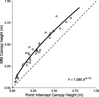
Figure 2. Canopy heights observed with point-intercept methods were positively correlated with canopy heights observed with structure-from-motion photogrammetry (SfM) at the plot level. Open circles represent observed values. The dotted line shows the 1:1 relationship for reference and the solid line is a power model. Mean canopy heights measured with SfM were consistently positively biased, on average by 0.14 m, relative to mean canopy heights measured with point-intercept.
Download figure:
Standard image High-resolution image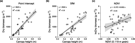
Figure 3. Aboveground biomass was strongly predicted by canopy height, but less strongly by NDVI. For each harvest plot, the mean canopy height was measured with point-intercept (a) and structure-from-motion photogrammetry (b), and mean NDVI was extracted from the 0.119 m grain raster (c). Linear models with constrained intercepts were fitted using least mean squares optimisation, with constrained intercepts for the canopy height models. The linear model fit is a simplification of the likely saturating relationships that we would expect to find across the full variation of NDVI and biomass values.
Download figure:
Standard image High-resolution image3.2. Canopy height explained variation in total biomass across plots
We found canopy height explained most of the variation in the aboveground biomass of vascular plants across the Salix richardsonii-dominated graminoid-shrub ecotone. The biomass models had slopes of 3623 ± 177 g m−1 and 2522 ± 143 g m−1, explaining 0.92 and 0.90 of the variance for point-intercept and SfM-derived canopy heights respectively (figure 3). Total aboveground biomass within the sampled plots ranged from 149 g m2 to 2431 g m2 with a mean of 1012 ± 699 g m2. Shrubs (woody material and leaves) accounted for the majority of biomass in 32 of the 36 plots. The biomass of shrub leaves was positively related to total biomass (slope = 19 g m−2) and explained 70% of the variation in total biomass (figure 5(a)). However, phytomass, calculated as the sum of shrub leaves and herbaceous material typically accounted for less than 10% of total biomass (figure S3), and did not correspond with total biomass (figure 5(b)). Herbaceous material (largely equisetum and some forbs) typically accounted for half of the phytomass in each harvest plot, ranging from 3% to 87% of the phytomass. The mass of leaf material was a reasonable predictor of total biomass (y = −63.7 + 19.04x; R2 = 0.70; figure 5(a)); however, phytomass was a poor predictor of total biomass (y = −1185−0.8471x; R2 = 0.01; figure 5(b)).
3.3. NDVI weakly explained variation in biomass
We found that NDVI positively corresponded with total aboveground biomass, phytomass and shrub leaf biomass (figures 3(c), 4 and S3, tables 2 and S2). However, NDVI explained less than a quarter of the variance in total aboveground biomass (14% to 23%), phytomass (2% to 7%) and leaf biomass (6% to 21%) across all four spatial grains investigated (figure 4, table 2). The predictive relationships weakened slightly as the spatial grain of the NDVI rasters became finer from 0.121 m to 0.018 m, with larger residual standard errors and smaller coefficients of determination (table 2). With a coarser spatial grain, the overall mean and variability amongst plot NDVI values was lower, although the relationship at the coarsest spatial grain (0.121 m) deviated slightly from this pattern (figure S4(a)). We speculate that this may relate to more pronounced bi-directional reflectance experienced during this particular drone survey that was conducted with a lower sun elevation of just 15.6 degrees (table 1). We tested whether the proportion of moss cover influenced the relationship between NDVI and total biomass, phytomass and the three biomass pools (table S3, figure S6), and though the interaction effects were similar with stronger NDVI-biomass relationships among plots with lower moss cover, the interaction was only significant (p < 0.05) for the phytomass relationship for the 0.121 m raster (figure 5(c)).
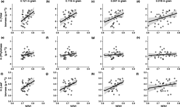
Figure 4. Mean NDVI was positively, but weakly related to total biomass, phytomass and leaf biomass at the plot level. Open circles represent observations, and black lines are linear models fitted to the log transformed biomass data described in table 2. Exponential models fitted to non-transformed biomass data are presented in figure S5 and table S2.
Download figure:
Standard image High-resolution image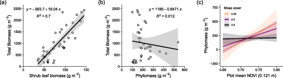
Figure 5. Shrubs are the dominant species in this landscape, and total aboveground biomass was predicted strongly by shrub leaf biomass, but not by overall phytomass. The mass of shrub leaves explained 70% of the variation in total biomass (a), but phytomass, calculated as the sum of shrub leaves and herbaceous material, explained none of the variation in total biomass (b). The proportion of moss cover only had a significant influence on the relationship between NDVI and phytomass for the 0.121 m grain raster (c). The relationship between NDVI and phytomass was strong when moss cover was low, but weakened as moss cover increased (See Figure S6 for non-significant interactions for other biomass pools and NDVI products).
Download figure:
Standard image High-resolution imageTable 2. Parameters of linear models fitted to mean plot normalised difference vegetation index (NDVI) and log-transformed total aboveground biomass, phytomass (leaf + herbaceous), and leaf biomass. In all cases the model form was ln(Y) = a + b X and n = 36. The standard error of the parameter is shown by ±.
| Dependent variable | Grain of NDVI in m | a | b | R2 | RMSE |
|---|---|---|---|---|---|
| Total biomass | 0.121 | −2.976 ± 2.987 | 13.04 ± 4.049 | 0.23 | 0.7162 |
| Total biomass | 0.119 | −0.372 ± 2.39 | 9.902 ± 3.373 | 0.20 | 0.7308 |
| Total biomass | 0.047 | 1.282 ± 2.244 | 7.412 ± 3.103 | 0.14 | 0.7571 |
| Total biomass | 0.018 | 2.909 ± 1.539 | 4.947 ± 2.037 | 0.15 | 0.7553 |
| Phytomass | 0.121 | 2.808 ± 1.479 | 3.307 ± 2.005 | 0.07 | 0.3547 |
| Phytomass | 0.119 | 3.464 ± 1.166 | 2.518 ± 1.646 | 0.06 | 0.3565 |
| Phytomass | 0.047 | 4.374 ± 1.082 | 1.207 ± 1.496 | 0.02 | 0.3651 |
| Phytomass | 0.018 | 4.664 ± 0.744 | 0.772 ± 0.985 | 0.02 | 0.3653 |
| Leaf biomass | 0.121 | 0.263 ± 1.428 | 5.54 ± 1.937 | 0.19 | 0.3426 |
| Leaf biomass | 0.119 | 1.213 ± 1.126 | 4.429 ± 1.589 | 0.19 | 0.3443 |
| Leaf biomass | 0.047 | 1.326 ± 1.005 | 4.183 ± 1.389 | 0.21 | 0.339 |
| Leaf biomass | 0.018 | 3.255 ± 0.754 | 1.45 ± 0.998 | 0.06 | 0.3703 |
To understand the performance of NDVI as a predictor of biomass, we examined the pairwise pixel covariance between NDVI and canopy height, as canopy height is a strong predictor of biomass (figure 6). We found a generally positive relationship between NDVI and canopy height, although the relationship was weaker at canopy heights below 0.2 m and once NDVI saturated at ca. 0.75. This relationship was consistent across all four spatial grains of NDVI sampled, and suggests NDVI-biomass transfer functions will be more uncertain where canopies are low (<0.2 m) or NDVI is high (>0.75). We used an NDVI-height transfer function developed by Bartsch et al (2020) to predict canopy height from NDVI and compare these predictions to photogrammetrically derived canopy height (figure S10), and found that while there was a generally positive relationship, the slope differed by a factor of ca. five. Models fitted to predict canopy height as a function of NDVI are reported in table S5.

Figure 6. Pairwise pixel covariance between NDVI and canopy height inferred from the photogrammetry for the monitoring area, both resampled to a common 0.25 m spatial resolution. There is a general positive relationship between NDVI and canopy height, although this breaks down at canopy heights below 0.2 m and once NDVI saturates at ca. 0.75. Models fitted to predict canopy height as a function of NDVI are reported in table S5.
Download figure:
Standard image High-resolution image3.4. Upscaling to landscape biomass estimations
We estimated aboveground vascular biomass density across the graminoid-shrub ecotone for the 0.5 ha−1 monitoring area (figure 1(d)). Estimated biomass at this landscape-level differed substantially between the five predictors, canopy height and NDVI at each of the four spatial grains (figure 6; table 3). We calculated the difference in estimated biomass relative to the CHM-derived biomass map, as we considered this to be the most accurate product (based on the model performance and our knowledge of this site). Although we consider the CHM-derived biomass estimate to be the most accurate, errors in the allometric model and in the canopy heights from the interpolated terrain model and plant surface model will all contribute uncertainty. For example, evaluation of the terrain model accuracy against 36 validation points indicated a mean residual elevation of 0.029 m ± SD 0.035 m. Although small, the systematic bias of 0.029 m in the interpolated terrain model (figure S7) amounts to 10% of the 0.278 m mean canopy height estimated for the monitoring area, and so would equals a 10% underestimate of biomass inferred from the CHM. The allometric models were fitted using similar distributions of canopy height and NDVI values to those found across the adjacent monitoring site. The distribution for the harvested samples of the two coarser NDVI rasters (0.121 m and 0.119 m) had slightly truncated tails, which may have contributed to greater uncertainty in the model fit (figure S8).
Table 3. Biomass density in the monitoring area estimated using the allometric equations obtained above. Lower and upper bounds are calculated using the standard errors for the equation coefficients (table S2).
| Predictor | Biomass (g m−2) | ||
|---|---|---|---|
| Best estimate | Lower bound | Upper bound | |
| CHM | 672 | 634 | 710 |
| NDVI 0.018 m | 972 | −128 | 26 704 |
| NDVI 0.047 m | 989 | −301 | 205 831 |
| NDVI 0.119 m | 1087 | −357 | 324 568 |
| NDVI 0.121 m | 1195 | −501 | 752 362 |
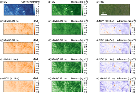
We found substantial differences in the estimated average biomass inferred from the five datasets (table 3). NDVI-based biomass estimates are generally greater than the height-based estimates (figures 7(f),(i),(l) and (o); figure S9), apart from areas with taller shrubs near the centre of the monitoring area. Estimated biomass was positively correlated with the spatial grain of the NDVI maps, mainly due to differences in the allometric models between different grain sizes (table S2, figure S5). However, the biomass estimates from NDVI were highly uncertain as demonstrated by the range of possible values (table 3).
Figure 7. Landscape-level biomass maps estimated from the canopy height model and NDVI for four spatial grains, using the allometric equations obtained above. Canopy height model (a), biomass-inferred from canopy height (b), RGB orthomosaic (c), NDVI reflectance (d), (g), (j), (m), biomass-inferred from NDVI *e),(h), (k), (n), and biomass difference maps relative to the biomass map inferred from canopy height (f), (i), (l), (o).
Download figure:
Standard image High-resolution image
4. Discussion
We found that canopy heights across a graminoid-shrub ecotone could be measured over fine (cm) spatial scales using structure-from-motion photogrammetry. Heights derived from drone photogrammetry corresponded strongly with those obtained using conventional point-intercept methods (figure 2) (Molau and Mølgaard 1996, Myers‐Smith et al 2019). Canopy heights were positively correlated with vascular plant biomass (figure 3), indicating that photogrammetry-derived data can be used to accurately estimate aboveground tundra biomass. However, vegetation greenness as measured by NDVI only weakly corresponded with vascular plant biomass and was influenced by the amount of moss cover on the ground (figure 5(c), figure S6). The relationship between fine-grain peak NDVI and biomass can be influenced by moss or other types of evergreen vegetation cover. Nonlinearity makes NDVI-biomass relationships particularly sensitive to the range and quality of the sample used to fit the curve. Our findings suggest that the relationship between fine-grain peak NDVI and biomass can be influenced by moss or other types of evergreen vegetation cover. Our study highlights that drone-derived canopy height can inform monitoring of vegetation change over larger and more representative extents, and thus improve projections of plant responses to warming in tundra ecosystems.
4.1. Photogrammetry-derived canopy heights were taller than in situ measured canopy heights
We found a positive bias in canopy heights measured with point-intercept relative to photogrammetry, which we attribute to differences in the way the two approaches quantify canopy architecture. The photogrammetry-derived heights in our study may have also been slightly exaggerated by slight depression at the plot corners by the survey staff on the ground surface at the top of the moss layer (ca. 2–3 cm) The plot-level terrain models will have smaller vertical errors than the model applied across the monitoring area (figure S7), because elevations were interpolated over smaller horizontal distances (<0.71 m). It is also possible that the fewer point-intercept observations within each harvest plot (n = 36) may under sample canopy structure relative to the photogrammetry (n ≈ 2500). Several studies have now reported strong correspondence between canopy heights reconstructed with photogrammetry and in situ measurements (Alonzo et al 2020, Karl et al 2020, Poley and Mcdermid 2020). For example, Clement and Fraser (2017) reported similarly good correspondence between in situ versus photogrammetrically derived maximum canopy heights for 20 shrubs measured at an Arctic tundra site near Iqaluktuuttiaq (Cambridge Bay). However, such comparisons are hindered by the sensitivity of maximum height measurements to outliers in these often noisy point clouds (Cunliffe et al 2016). The comprehensive review by Poley and Mcdermid (2020) discusses such inter-comparisons of different canopy height measurements in further detail, but they were unable draw general conclusions because all sets of observations are sensitive to the ways in which they are collected, processed and analysed (Cunliffe et al 2016, Wallace et al 2017, Fraser et al 2019). Our findings suggest that, when applied in a consistent manner, drone photogrammetry is an appropriate tool for monitoring shrub canopy heights in such ecosystems.
4.2. Canopy heights predicted aboveground biomass
Canopy height strongly predicted aboveground biomass for the Salix richardsonii-dominated community that we studied, which corroborates similar reports for photogrammetry across a range of biomes and plant communities (Bendig et al 2015, Selsam et al 2017, Grüner et al 2019, Wijesingha et al 2019, Alonzo et al 2020, Howell et al 2020, Karl et al 2020). Estimating aboveground biomass from canopy height models depends on having an underlying terrain model of sufficient quality to describe topographic variability (Cunliffe et al 2016, Fraser et al 2019, Poley and Mcdermid 2020). In this study, we derived our terrain model using RTK-GNSS observations, which can be a viable option for characterising topography over extents of up to a few hectares. In ecosystems where canopies are spatially or temporally discontinuous, terrain models could also be derived directly from photogrammetric point clouds (Cunliffe et al 2016, Fraser et al 2019). Terrain models derived using other survey techniques could also be co-registered in a hybrid approach (Dandois and Ellis 2013). However, propagation of uncertainties including co-registration error is vital for understanding the limits of detection of genuine change in canopy height (James et al 2017).
4.3. Refining predictions of biomass from canopy height
Relationships between plant dimensions and biomass are sensitive to the ways in which these measurements are obtained (Cunliffe et al 2020). Cross-site data syntheses therefore require the use of standardised protocols for data collection and processing (such as HiLDEN https://arcticdrones.org/, Assmann et al 2018, Cunliffe and Anderson 2019). As noted by Pätzig et al (2020), there is a need for further coordinated work to calibrate the relationship between photogrammetric-inferred canopy height and aboveground biomass for different taxonomic groups. There is also a need to quantify the sensitivity of these relationships to key parameters (e.g. the spatial resolution of the input data, the implementation of multi-view stereopsis and the spatial grain of analysis, sensu Zarco-Tejada et al 2014, Wallace et al 2017), as well as to differences in environmental conditions (e.g. illumination and wind-induced movement of plant canopies, Dandois et al 2015, Frey et al 2018).
4.4. Vegetation greenness only weakly corresponded with biomass
We found that NDVI only weakly predicted the aboveground biomass of vascular plants, explaining at most 23% of the variation in total biomass, and even less of the variance in phytomass or leaf biomass (figures 4 and S3, tables 2 and S4). Inferring aboveground biomass from NDVI is predicated on the assumptions that (i) NDVI is a good predictor of phytomass, and (ii) that phytomass is a good predictor of total biomass. We found that while NDVI had some capacity to explain variance in phytomass (figure 4, table 2), phytomass was a very weak predictor of total biomass (figure 5(b)). Across spatial grains, predictive relationships weakened slightly as the spatial grain of the NDVI rasters became finer from 0.121 m to 0.018 m (table 2). We attribute two main causes for the weak correspondence between NDVI and biomass. Firstly, although leaf biomass was a strong predictor of total aboveground biomass, leaf biomass accounted for typically only half of the phytomass in each plot, and phytomass (including herbaceous material and shrub leaves) only weakly corresponded with total biomass (figure 5). Vegetation indices that integrate all photosynthetically active material are often poor predictors of total biomass (Bratsch et al 2017, Räsänen et al 2019). Secondly, we found indications that moss cover influenced the relationship between NDVI and phytomass. The direction of the relationship was consistent; however, the interaction effect was only statistically significant in one of the 12 combinations of NDVI raster and biomass pool tested (table S3). We found that the relationship between NDVI and vascular phytomass was mediated by the amount of moss cover beneath the sampled vegetation and weakened as moss cover increased (figures 5(c) and S6). Vegetation species composition therefore affects the biomass NDVI-relationship.
The relationship between NDVI and biomass in this tundra setting is approximated by the relationship between NDVI and canopy height across the monitoring site. NDVI was generally positivity related to canopy height across all four NDVI rasters (figure 6); however, the relationship was very weak at canopy heights below 0.2 m and NDVI values above ca. 0.75. NDVI-biomass transfer functions will thus be more uncertain where canopies are low (<0.2 m), in some cases due to increased signal from bryophytes, or where NDVI reaches saturation at around 0.75. Canopy heights inferred from NDVI using the NDVI-height transfer function developed by Bartsch et al (2020) were linearly related to canopy heights inferred from photogrammetry, although were positively biased by a factor of ca. five and subject to the same issues around the shorter (<0.2 m) canopies and NDVI saturation. This bias suggests that NDVI-biomass transfer functions will need to be calibrated more specifically for different situations.
The weak correspondence between NDVI and phytomass that we observed contrasts with reports of stronger positive relationships between NDVI and aboveground biomass derived from datasets compiled across different spatial scales (Boelman et al 2003, Walker et al 2003, Goswami et al 2015). NDVI has a saturating relationship with biomass and NDVI-biomass relationships can be confounded by a variety of ecological variables, land-surface properties and view angle effects (Walker et al 2003, Buchhorn et al 2016, Karlsen et al 2018, Myers-Smith et al 2020). Our findings are consistent with the well-known saturation effect (e.g. Berner et al 2018), and we may have found better correspondence between NDVI and biomass if we had sampled over a wider range of NDVI values beyond those that were most prevalent at our study site. The unmeasured biomass associated with moss was likely small compared with the biomass associated with the vascular plants at this site (Reid et al 2012), but if we had included moss in our biomass harvests, this might have modified relationships between NDVI and biomass. Our results highlight the need for caution when deriving total biomass maps from vegetation indices in high latitude ecosystems with variable land cover. The biome-wide tundra greening patterns and trends observed with large-grain satellite datasets are unlikely to directly represent plant functional attributes such as canopy height or biomass in situ (Myers-Smith et al 2020). Thus, to improve our understanding of vegetation greening in tundra ecosystems across vegetation types and geographic gradients, we need data collection across scales from focal sites to the tundra biome (Fisher et al 2018, Miller et al 2019, Myers-Smith et al 2020).
4.5. Landscape-estimates of biomass
The spatially continuous estimates of canopy height and inferred vascular plant biomass across our monitoring site (figure 6, table 3) are well suited for upscaling studies. These kinds of highly accurate and precise products help to overcome limitations with incomplete characterisations of plant communities due to labour intensive and resource limited in situ monitoring programs (Myers‐Smith et al 2019, Alonzo et al 2020, Bartsch et al 2020). Of particular concern are the difficulties comparing observations from very different spatial extents, between remotely-sensed observations and small, potentially non-representative in situ plots. Biomass estimated from NDVI was highly uncertain (table 3), even when only accounting for uncertainty in the coefficients of our exponential models without accounting for uncertainties in the NDVI values themselves. Drone-derived products are useful for calibrating and validating biomass retrievals of these properties from coarse-scale observations, and for testing key of assumptions underpinning novel retrievals approaches (Bartsch et al 2020). Photogrammetric approaches to monitoring plant canopies can also be deployed over even larger extents using similar data from airborne surveys (Alonzo et al 2020).
5. Conclusion
This study expands the empirical understanding of how fine-grained remotely-sensed observations relate to vegetation attributes. By comparing structural, spectral reflectance and on-the-ground ecological metrics, we can improve our understanding of the scaling relationships from fine- to coarse-scale observations of tundra vegetation change. Drone-collected data are already helping us to fill in the missing landscape-scale gap in tundra ecological monitoring, and future work must use coordinated protocols to underpin biome-scale data synthesis (e.g. HiLDEN https://arcticdrones.org and Cunliffe and Anderson 2019). We found strong agreement in canopy heights measured using in situ point-intercept methods compared to drone-photogrammetry. Canopy height was strongly and linearly related to the aboveground biomass of vascular plants, explaining ca. 90% of the observed variability in the biomass. Vegetation 'greenness' measured as NDVI across four independent multispectral surveys explained only a small proportion of the variability in the biomass of vascular plants and was influenced by moss cover, suggesting caution should be used when attributing differences in NDVI to differences in either vascular plant biomass or phytomass. Our comparison of structural, spectral and in situ ecological measurements contributes to improved understanding of tundra vegetation as inferred from remote sensing and thus informs monitoring of vegetation change in a warming tundra biome.
Acknowledgments
This work was supported by NERC ShrubTundra project (NE/M016323/1), and the loan of GNSS equipment from NERC GEF (NERC/GEF: 1063 and 1069). JTK received funding from the Neukom Institute at Dartmouth College, The Aarhus University Research Foundation, and the European Union's Horizon 2020 research and innovation programme (Marie Skłodowska-Curie grant: 754513). The authors wish to thank the Inuvialuit people for permission to work on their lands, and the Yukon Government and Parks for their permission and logistical support for this research (Yukon Scientists and Explorers license: S&E16–48; Parks Permit number Inu-02-16). We thank the Herschel Island–Qikiqtaruk Territorial Park rangers for logistical support of this research. Drone flight operations were authorised by a Special Flight Operations Certificate granted by Transport Canada (RDIMS: 11956834). We thank Tom Wade and Simon Gibson-Poole from the University of Edinburgh's Airborne GeoScience Facility and Brenden Duffy from ConservationDrones.org for their advice and assistance with the drone platforms used in this study. We thank Haydn Thomas, Sandra Angers-Blondin, Eleanor Walker, John Godlee and Santeri Lehtonen for assistance with fieldwork.
Statement of contribution
AMC and IHM-S conceived the research idea. AMC, JJA and IHM-S developed the experimental design. IHM-S acquired the funding. AMC, JJA, JTK and IHM-S undertook the investigation. AMC and GND completed the analysis, and AMC, JJA and GND completed the data visualisation. AMC led the writing of the manuscript. All authors contributed to the final version of the manuscript.
Data accessibility
The data that support the findings of this study are openly available at the following DOI: https://doi.org/10.5285/61C5097B-6717-4692-A8A4-D32CCA0E61A9).
Conflicts of interest
The authors declare no conflicts of interest.