

Abstract
Changes in mean sea level (MSL) are a major, but not the unique, cause of changes in high-percentile sea levels (HSL), e.g. the annual 99.9th quantile of sea level (among other factors, climate variability may also have huge influence). To unravel the respective influence of each contributor, we propose to use structural time series models considering six major climate indices (CI) (Artic Oscillation, North Atlantic Oscillation, Atlantic Multidecadal Oscillation, Southern Oscillation Index, Niño 1 + 2 and Niño 3.4) as well as a reconstruction of MSL. The method is applied to eight century-long tide gauges across the world (Brest (France), Newlyn (UK), Cuxhaven (Germany), Stockholm (Sweden), Gedser (Danemark), Halifax (Canada), San Francisco (US), and Honolulu (US)). The treatment within a Bayesian setting enables to derive an importance indicator, which measures how often the considered driver is included in the model. The application to the eight tide gauges outlines that MSL signal is a strong driver (except for Gedser), but is not unique. In particular, the influence of Artic Oscillation index at Cuxhaven, Stockholm and Halifax, and of Niño Sea Surface Temperature index 1 + 2 at San Francisco appear to be very strong as well. A similar analysis was conducted by restricting the time period of interest to the 1st part of the 20th century. Over this period, we show that the MSL dominance is lower, whereas an ensemble of CI contribute to a large part to HSL time evolution as well. The proposed setting is flexible and could be applied to incorporate any alternative predictive time series such as river discharge, tidal constituents or vertical ground motions where relevant.
Export citation and abstract BibTeX RIS

Original content from this work may be used under the terms of the Creative Commons Attribution 3.0 licence. Any further distribution of this work must maintain attribution to the author(s) and the title of the work, journal citation and DOI.
1. Introduction
Changes in extreme sea levels are recognized mainly driven by variations in mean sea level (MSL), as pointed out in the 2013 IPCC report (IPCC 2013). Previous studies have shown and extensively documented the relation between variability and trends in extremes and MSL; see for instance, Menéndez and Woodworth (2010), Woodworth et al (2011), Wahl and Chambers (2015). However, MSL being the major contributor does not necessarily mean that it is the only one. Today, extreme sea level events associated with storm surges are already prominent threats for populations and ecosystems on the coasts. The combination of such extreme events with MSL rise and the related damages are a significant concern (Wahl 2017) for present day and for the future. Therefore, planning adaptation strategies (like hard protection, soft protection, accommodation, retreat) and designing protective infrastructures (like dikes, and seawalls) for the future both require improving the understanding and the predictability of such extreme events via a deeper knowledge of their drivers.
On top of the MSL, forcing related to ocean and atmosphere variations influence extreme sea levels at inter-annual and decadal time scales. To investigate such large-scale climate variability, climate indices (denoted CI) like North Atlantic Oscillation (NAO) or Atlantic Multidecadal Oscillation (AMO) have been used; see e.g. Menéndez and Woodworth (2010), Woodworth et al (2011), Talke et al (2014), Marcos et al (2015), Wahl and Chambers (2015, 2016), Mawdsley and Haigh (2016), Marcos and Woodworth (2017), Wong et al (2018). Far from being theoretical, these research studies bring societal benefits. First, understanding and quantifying the role of each influencing factor is a prerequisite to a formal detection and attribution of coastal extreme water levels, which is a perceived important to stimulate mitigation of climate change (Schwab et al 2017). Second, assuming that MSL is the only driver of extreme sea levels, and neglecting the influence of other evolving factors such as CIs, might reduce confidence in current estimates and future projections of extreme coastal water levels, and might even mislead coastal adaptation practitioners in the worst case.
The most widespread method to address the problem of controls on extreme sea levels is the use of linear (Pearson) correlation coefficients (e.g. Marcos and Woodworth (2017): section 4) with possible combination with significance testing techniques. Though efficient and easy-to-implement, this approach remains global and does not account for: (1) the nature of the data, which are time series i.e. the considered time series may be correlated at different time instants; (2) multiple possible drivers (i.e. predictors), which may act in interaction. To overcome both limitations, Wahl and Chambers (2016) proposed the use of multiple regression models. Yet, this approach ignores structural uncertainty, which arises when different alternative models can be proposed to explain the data and appear 'equally appropriate' from a statistical perspective.
A possible option for handling this type of uncertainty is to fit a multiple regression model within a Bayesian setting, which enables to examine a large number of possible variable configurations with respect to the observations (Hoeting et al 1999). The Bayesian treatment of the fitting process then provides an importance measure (here the posterior inclusion probability as defined for instance by Scott and Varian 2014), which measures how often each driver is included in the regression model. This is can be used to unravel the respective influence of each driver of extreme sea levels.
In the present study, we propose to rely on this Bayesian approach to quantify the respective contribution of the different drivers to the time evolution of high-percentile sea levels (denoted HSL), such as 99 or 99.9th quantile, over inter-annual to centennial timescales. Multiple possible predictors are accounted for, namely, the annual MSL and six large-scale CI (see further details in section 2). A more advanced method for time series modelling than multiple regression modelling is chosen, namely the technique of Bayesian structural time series model (denoted bsts in the following), as developed by Scott and Varian (2014, 2015), which is particularly flexible to model the complex multivariable, correlational structure of any temporal data.
The paper is organised as follows. In a first section, we describe the century-long sea level time series used for the study, the pre-processing that we conducted and the CI. In a second section, we provide full details of the proposed procedure based on bsts method. In section 4, we analyse and discuss the results of the procedure applied to eight tide gauges across the world.
2. Data
We have extracted from the Global Extreme Sea Level Analysis (GESLA, version 21 , Woodworth et al 2017) tide gauge data repository, eight of the longest (quasi century-long) time series of sea levels sampled at a hourly frequency, namely: Brest, France (1846–2014); Newlyn, UK (1915–2014); Cuxhaven, Germany (1918–2015); Gedser, Danemark (1891–2012); Stockholm, Sweden (1889–2012); Halifax, Canada (1920–2011); San Francisco, US (1897–2012); Honolulu US (1905–2012). See locations in supplementary materials, available online at: stacks.iop.org/ERL/14/014008/mmedia.
These data present very limited missing values except for Brest for the time interval between 1943–1953 and for Stockholm for the year 1982. These missing data were replaced by means of an imputation approach based on a Kalman smoothing approach (see e.g. Moritz and Bartz-Beielstein 2017). The impact of this choice on the results presented in section 4 was tested by using other imputation approaches (mean value, linear interpolation, etc), but appears to be very limited (see supplementary materials). We adopted the percentile time series analysis described by Woodworth and Blackman (2004), and we extracted the annual 99.9th percentile from the hourly SL data. Note that the annual 99.9th percentile approximately corresponds to the level of the eight highest hourly sea level values over the considered year. This constitutes the annual HSL time series used in the following. The influence of the quantile level is investigated in section 4.3.
The annual MSL was estimated at each time step by post-processing the annual data provided by PSMSL2 using a forward–backward Kalman-filter (e.g. Visser et al 2015); see further details in supplementary materials. This procedure allows separating nonlinear changes in MSL from inter-annual modes of variability, which are part of the residual signal to be detected in HSL time series. Figure 1 shows the different time series for the eight locations. Note that the scaling between MSL and HSL are different due to differences in the processing (reference value, detrending and scaling) of both dataset (i.e. from PSMSL and from GESLA).
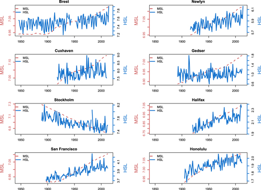
Figure 1. Time series of annual mean sea level MSL, in meters (red line) and high-percentile (at 99.9th) sea level HSL, in meters (blue line) for the eight tide gauges considered in the present study. MSL is derived from the PSMSL dataset using a Kalman-filter approach; HSL is post-processed from the global extreme sea level analysis (GESLA, version 2) tide gauge data repository. Note that the scaling between MSL and HSL are different due to differences in the processing (reference value, detrending and scaling) of both dataset (i.e. from PSMSL and from GESLA).
Download figure:
Standard image High-resolution imageTable 1 provides the source of the CI selected in the present study. Six major CI were selected, namely NAO, AMO, Arctic Oscillation (AO), Southern Oscillation Index (SOI), Niño 1 + 2 SST Index (NINO12), and Niño 3.4 SST Index (NINO34). These indices were selected because previous studies have shown their role in controlling HSL variability (e.g. Marcos et al 2015), and because the time series currently available are in the order of 150 years (with a starting date before 1900) and therefore allow to detect the influence of predictors at low frequency (table 1). The monthly time series are converted to annual data by taking the mean value for each year. The starting date is selected as the maximum value between the CI' times series and the considered MSL data (in figure 2, it corresponds to 1915 in the Newlyn case).
Table 1. Climate indices selected in the present study.
| Climate index | Starting date | Source (last access on 19/09/2018) |
|---|---|---|
| North Atlantic Oscillation (NAO) | 1821 | https://esrl.noaa.gov/psd/gcos_wgsp/Timeseries/NAO/ |
| Atlantic Multidecadal Oscillation (AMO—smoothed version) | 1861 | Enfield et al (2001), Rayner et al (2003) |
| https://esrl.noaa.gov/psd/gcos_wgsp/Timeseries/AMO/ | ||
| Arctic Oscillation (AO) | 1871 | https://esrl.noaa.gov/psd/gcos_wgsp/Timeseries/Data/ao20thc.long.data |
| Southern Oscillation Index (SOI) | 1866 | Ropelewski and Jones (1987), Allan et al (1991), Können et al (1998) |
| https://esrl.noaa.gov/psd/gcos_wgsp/Timeseries/SOI/ | ||
| El Nino 12 | 1870 | Rayner et al 2003 |
| https://esrl.noaa.gov/psd/gcos_wgsp/Timeseries/Nino12/ | ||
| El Nino 34 | 1870 | Rayner et al 2003 |
| https://esrl.noaa.gov/psd/gcos_wgsp/Timeseries/Nino34/ |

Figure 2. Time series of annual mean for six different climate indices (see table 1). The starting date is selected as the maximum value between the climate indices' times series and the considered MSL data (here Newlyn tide gauge).
Download figure:
Standard image High-resolution image3. Method
We aim at modelling the observed HSL series by accounting for two sources of information, namely: (1) the time series behaviour of HSL prior to the considered time instant (i.e. the trend); (2) the behaviour of other (control) time series that is known to be predictive of HSL, namely MSL and d different climate indices CI1,...,d (here termed as the predictors). Both sources of information are combined using a structural time series model trained within a Bayesian setting denoted bsts (full details are provided by Scott and Varian 2014) as follows:

where β are the regression coefficients (with β0 a constant value termed as intercept), which are related to MSL and the d CI. The noise term  follows a zero-mean Gaussian distribution with fixed standard deviation σt and is assumed to be independent from the other parameters (i.e. the evolution is driven by an independent Gaussian random walk).
The term  at time instant t is modelled via a 1-lag autoregressive model:

where  follows a zero-mean Gaussian distribution (with fixed standard deviation σμ), and is independent from the other parameters; ϕ are the regression coefficients.
The model fitting is conducted within a Bayesian setting, which allows accounting for empirical priors on the afore-described parameters (i.e. the regression coefficient ϕ1, the regression coefficients β and the different variance parameters of the error terms ε) and the initial states (i.e. the term  and the predictors).
A spike-and-slab prior is assumed to express a prior belief that a sparse set of variables can explain the response, i.e. that most of the regression coefficients β are exactly zero (Scott and Varian 2015). Full details on the regressor priors' definition and parametrisation are provided in supplementary materials. The full model is estimated via a Bayesian model averaging procedure (Hoeting et al 1999), which combines information from the priors and uses a Markov chain Monte Carlo procedure (see technical details in Scott and Varian 2014: section 4). A space of large number (typically 1000–10 000) of likely variable configurations that explain the response are computed using Gibbs sampling techniques and treated within a stochastic search variable selection framework (George and McCulloch 1993).
From the random sampling procedure, the marginal posterior inclusion probability for each predictor can be evaluated, i.e. the proportion of Monte Carlo draws with a regression coefficient β ≠ 0. This means that the inclusion probability measures how often each predictor is selected during the Monte Carlo procedure. Thus, the larger the inclusion probability, the larger the influence of the considered predictor. By using the bsts-derived inclusion probability, it is then possible to measure the influence of each driver (MSL or CI) while accounting for the complex multivariable (i.e. presence of multiple predictors), correlational structure (i.e. we are dealing with time series) of the data.
The capability of the bsts model to reproduce the observations over the considered time period is measured using the coefficient of determination (denoted R2) considering the error between the posterior predictive mean for the modelled (denoted  ) and the observed HSL as follows:
where  is the average value of HSL over the considered time interval. If R2 is close to 1, this means that the posterior predictive mean of the bsts model explains almost the whole HSL variability.
In practice, the bsts model is fitted using the R package called 'bsts' available at: https://cran.r-project.org/web/packages/bsts/index.html
4. Application
4.1. Application to Newlyn tide gauge
To illustrate the different steps described in section 3, the procedure is first applied to the Newlyn tide gauge. All time series (HSL, MSL, and CI) are first standardized, i.e. the mean was subtracted and the time series was divided by their respective standard deviation. The evolution of the observed (standardized) HSL is modelled using the afore-described bsts approach by using 10 000 random draws (figure 3). The influence of the number of random samples is investigated in supplementary materials.
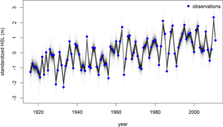
Figure 3. Fit of the bsts model to the observed HSL (standardized) at Newlyn tide gauge. The blue dots are the observations. The posterior median is colored black, and each 1% quantile away from the median is shaded slightly lighter, until the 99th and 1st percentiles are shaded white.
Download figure:
Standard image High-resolution imageThe coefficient of determination R2 here reaches values larger than 90% with a full coverage of the 99% posterior predictive intervals, hence yielding very satisfactory goodness of fit.
Figure 4 displays the posterior inclusion probability and shows that for all of 10 000 random draws, MSL is almost systematically selected (inclusion probability of nearly 100%), hence confirming the dominant influence of MSL to explain changes in HSL. The two other important drivers of HSL time evolution appears to be the NAO and AO with inclusion probability values of respectively 37% and 33%. The bars are shaded on a continuous [0, 1] scale in proportion to the probability of a positive coefficient, so that negative coefficients are black, positive coefficients are white, and gray indicates indeterminate sign. This shows that MSL has a positive relationship with HSL (i.e. positive effect), whereas NAO and AO have a negative one.
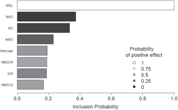
Figure 4. Inclusion probability derived from the bsts model fitted to the 99.9th percentile of sea levels at Newlyn tide gauge over a time period with final date of 2011. This figure allows identifying the influence each contributor HSL evolution (see method section). The colorbar corresponds to the probability of positive effect, i.e. negative relationship with HSL are black, positive ones are white, and gray indicates indeterminate sign. The term Intercept corresponds to a constant scalar value in equation (1).
Download figure:
Standard image High-resolution image4.2. Application to the set of tide gauges
The procedure described for Newlyn is performed for the seven other tide gauges using 10 000 random samples. The influence of the number of samples is tested in supplementary materials. The starting date is selected as the maximum value between the CI times series and the considered MSL data and the final date is 2011. The goodness of fit of the bsts model is checked for each tide gauge, which shows that the R2 coefficient reaches for all cases values of around 90% (see the fitted models in supplementary materials).
Figure 5 presents the inclusion probability for each tide gauge. Several observations can be made.
- •
- •For Brest, Newlyn and Honolulu, the CI contribution remains low-to-moderate with an inclusion probability not larger than ≈40%, hence indicating that MSL is the main driver.
- •No particular tendency can be identified for Gedser, where all predictors (MSL and CI) appear to have a low-to-moderate inclusion probability of the order of 20%.
- •For Cuxhaven, Stockholm, Halifax, and San Francisco, a combination of two drivers exist, namely MSL + AO for the three first tide gauges, and MSL + NINO12 for the latter. The inclusion probability of the CI is larger than 90%, i.e. as large as the one of MSL or even larger at Cuxhaven. The sign of the AO effect is positive for Cuxhaven and Stockholm, but negative for Halifax. The difference in the sign effect may be related to the location of each tide gauges with respect to the sea level anomalies characterizing AO in North Atlantic, which corresponds to a positive pattern at latitudes 37°–45° N (Halifax latitude is 44.6° N) and a negative above 45° N (Cuxhaven and Stockholm latitudes are 53.8° N and 59.3° N).
- •Surprisingly, our study little highlights NAO as a strong driver at the exception for Newlyn contrary to previous studies, (e.g. Marcos and Woodworth 2017). A possible explanation is the strong relationship between AO and NAO (e.g. Ambaum et al 2001) so that the signal held by NAO may be 'viewed' as redundant with the one of AO by the bsts model.
- •A clear evidence of strong Niño 1 + 2 SST influence is evidenced at San Francisco. This appears consistent with conclusions of different studies on the link between extreme coastal response and El Niño events (see e.g. Barnard et al 2017 and references therein).

Figure 5. Inclusion probability derived from the bsts model fitted to the 99.9th percentile of sea levels for all tide gauges over a time period before 2011. The colorbar corresponds to the probability of positive effect, i.e. negative relationship with HSL are black, positive ones are white, and gray indicates indeterminate sign. The term Intercept corresponds to a constant scalar value in equation (1).
Download figure:
Standard image High-resolution image4.3. Influence of the assumptions
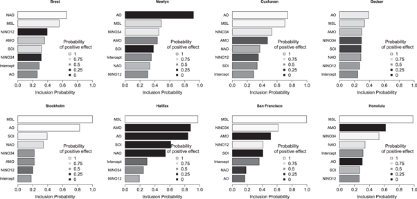
In this section, we investigate the implications of two assumptions. First, the length of the training time period is investigated. In section 4.2, the dominance of MSL and of AO and NINO12 was identified over a time-period with a final date of 2011; we now investigate the prevalence of this influence in the first half of the 20th century, i.e. when the final date is set at 1950. Figure 6 shows that the corresponding inclusion probability values have largely changed from the ones of figure 5. Clearly, the large dominance of MSL has decreased for most tide gauges; in particular, the inclusion probability of MSL has lowered to 40%–60% at Brest, Newlyn, Cuxhaven, and Halifax. Contrary to the analysis on the whole time period before 2011, the HSL evolution before 1950 appears to be driven not only by two predictors, but by an ensemble of them as exemplified at Halifax, where both AO and SOI have a large influence with inclusion probability larger than 60%. For Stockholm, San Francisco, and Honolulu, the large dominance of MSL persists before 1950, but with larger influence of other CI, whose inclusion probability values are of the order of 60%. For Gedser, a larger dominance of AO is identified before 1950. A possible interpretation holds as follows. During the 20th century, MSL is rising at all stations considered in this study, except for Stockholm. This means that extreme sea levels are more influenced by the cumulative effects of sea level rise during the 2nd half of the 20th century than during earlier periods of time. Furthermore, it can be noticed that the longest time series (Brest) includes records before the onset of sea level rise, during which the influence of NAO is expected to be prominent, as quantitatively confirmed in figure 6 (top left panel).
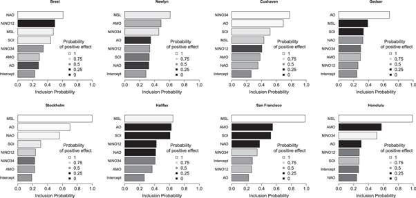
Figure 6. Inclusion probability derived from the bsts model fitted to the 99.9th percentile of sea levels over a time period before 1950. The colorbar corresponds to the probability of positive effect, i.e. negative relationship with HSL are black, positive ones are white, and gray indicates indeterminate sign. The term Intercept corresponds to a constant scalar value in equation (1).
Download figure:
Standard image High-resolution imageSecond, we analyse whether the dominance of MSL still prevails when the threshold chosen to select HSL events is lowered, e.g. down to 99% (approximately corresponding to the level of the 90 highest hourly sea level values over the considered year). Figure 7 shows that the conclusions drawn from figure 5 are no longer valid for most tide gauges at the exception of Cuxhaven (which still presents a dominant combined role of AO and MSL) and at Gedser (where hardly any tendency can be identified). The decreased influence of MSL is noticeable for Stockholm, Halifax, San Francisco and Honolulu with a clear increased influence of different CI. For instance, at Halifax, AMO and AO both have inclusion probability larger than 80%. For Brest and Newlyn, the influence of MSL appears to be diminished in comparison to the one of NAO and AO respectively.
Figure 7. Inclusion probability derived from the bsts model fitted to the 99.0th percentile of sea levels over a time period with final date of 2011. The colorbar corresponds to the probability of positive effect, i.e. negative relationship with HSL are black, positive ones are white, and gray indicates indeterminate sign. The term Intercept corresponds to a constant scalar value in equation (1).
Download figure:
Standard image High-resolution image
The sensitivity to the threshold chosen to select extreme sea level can be related to a physical explanation. Since this threshold is lowered from the annual 99.9th to the annual 99th percentile, the number of events included in the analysis is increased. Consequently, HSL time series corresponding to the lowest quantile reflect more persistent storm weather conditions, which are themselves more apparent in the mean annual CI (e.g. Seierstadt et al 2007). Hence, although consistent with an intuitive analysis, the results presented in figures 5 and 7 confirm quantitatively that the influence of CI increases when lowering the threshold for selecting extreme sea level.
5. Concluding remarks and further work
The proposed approach based on structural time series modelling provides a rigorous setting for measuring the importance of MSL in the evolution of HSL. The proposed procedure in combination with a Bayesian treatment of the fitting process enables to deal with the limitations of current available procedures, namely: (1) the presence of multiple alternative drivers; (2) the temporal nature of the data and (3) the uncertainty in the model construction. By applying bsts modelling procedure, we evaluate the inclusion probability, which measures how often a given driver is included in the regression model to explain HSL. This shows that, for the considered tide gauges, the MSL signal dominates the HSL evolution (except for Gedser). This result is in agreement with past studies, which have outlined the key role of MSL in extreme sea levels (see for instance the recent study by Marcos and Woodworth 2017). Interestingly, the MSL influence is clearly limited when the analysis is conducted before 1950, hence indicating a more marked influence of MSL on HSL as the cumulated amount of sea level rise increases (except for Stockholm). Our study also highlights that MSL is not the only and unique contributor. This is particularly evidenced at three tide gauges where AO index appears to have strong influence, but with opposite effect, namely positive at Stockholm and Cuxhaven and negative at Halifax. A clear evidence of strong Niño 1 + 2 SST influence is also evidenced at San Francisco, which appears to be consistent with the city location on the west coast of the US. These results may also suggest a connection between the climate driver and the considered tide gauge's location (see e.g. Woodworth et al 2011, Marcos et al 2015), i.e. Pacific North American tide gauges are more likely be dominated by indices characterizing El Niño and European tide gauges are more likely be influenced by major climate modes of the Atlantic North Ocean. Marcos et al 2015 also reported identification of significant correlation to 'remote' CI (e.g. correlation of San Francisco extreme to NAO). Similar 'remote' influence of CI on storminess have been identified earlier by Seierstadt et al (2007). To some extent, they are evidenced by the bsts model as well, but mostly until 1950. Overall, our results suggest that the bsts model behaves more robustly as it identifies only a couple of important drivers, which remain consistent with the considered location.
In the present study, we have focused on measuring the importance of MSL and CI in the HSL time signal. Yet, sea level time series at tide gauges are known to be the complex result of different phenomena in interplay (in addition to MSL) including: (1) multidecadal variability related to CI. The present study focused on six major CI, but other could be easily integrated and in particular new CI specifically developed for the purpose of HSL variability study (as Wahl and Chambers 2016 did); (2) effects of river flows (in estuaries, see e.g. Piecuch et al 2018) and evolving complex nonlinear shallow water processes, affecting the tidal levels and constituents (Woodworth 2010), as evidenced for instance in the northern part of the German Bight (Arns et al 2015) or along the US coasts (e.g. Ray 2009); (3) nonlinear vertical ground motions (e.g. Raucoules et al 2018) (4) technological artifacts such as modification in the protocol for data acquisition errors (e.g. Woodworth 2010).
Incorporating other predictive time series related to additional physical processes driving extreme sea levels constitutes a line for future research. This is made possible owing to the high flexibility of the proposed setting whatever the type and number of predictive time series.
Acknowledgments
We acknowledge financial support of Project EUPHEME, which is part of ERA4CS, an ERA-NET initiated by JPI Climate, and funded by FORMAS (SE), BMBF (DE), BMWFW (AT), IFD (DK), MINECO (ES), ANR (FR) with co-funding by the European Union (Grant 690462). We thank Robert Vautard, Pascal Yiou and Marta Marcos for useful discussions on attribution techniques and extreme sea levels time series at tide gauges. We thank two reviewers for their comments that led to a significant improvement of the article.