

Export citation and abstract BibTeX RIS

Original content from this work may be used under the terms of the Creative Commons Attribution 3.0 licence.
Any further distribution of this work must maintain attribution to the author(s) and the title of the work, journal citation and DOI.
Due to processing errors, the appendices were omitted from the original article. In addition, references to the appendices require amendment as follows. In section 2.3., paragraph 3, there are two sentences which currently read as 'Details on the generation of the climate scenario data are provided in appendix C. Details on the analysis, including data transformations and the use of 2 way ANOVA, are provided in appendix D.' These should be replaced with: 'Details on the generation of the climate scenario data are provided in appendix B. Details on the analysis, including data transformations and the use of 2 way ANOVA, are provided in appendix C.'
The appendices should appear as below.
Appendix A. Equations governing P loss and transport
A.1. Dissolved P loss in runoff
For dissolved P loss, the equations in Agro-IBIS come from the SurPhos model which estimates daily amounts of dissolved P loss from manure, fertilizer, and soil (Vadas et al 2007). The calculation for dissolved P loss from manure is comprised of the following equations.

where DPman is the concentration of dissolved P in runoff from manure (mg L−1), RAIN is daily rainfall (mm), AREA is the grid-cell area (ha), and LCHm is water extractable P leached from dairy manure (kg), calculated as:
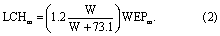
WEPm is the pool of water extractable P in manure (kg), and W is the water to soil ratio (mL g−1), calculated as:
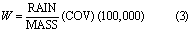
where MASS is current manure dry matter mass (kg), and COV is the current area covered by manure (ha). The P distribution factor, PDFACTOR, is calculated as:

where RUNOFF is daily runoff (mm).
Equations (1)–(3) were originally based on relationships governing P desorption from soil to water developed by Sharpley et al (1981), which showed a dependence on the water-to-soil ratio as well as the time of interaction between water and soil. Kleinman et al (2002a) showed that these concepts applied well to P losses from dairy, swine, and poultry manures in lab experiments. Subsequently, Vadas et al (2004) used data from several sources (Sharpley and Moyer 2000, Kleinman et al 2002b, 2004, Kleinman and Sharpley 2003) as well as their own runoff box experiment to improve the equations as they apply to manure, and modify them to accommodate daily time-step models. The updates included a variable runoff-to-rainfall ratio factor (PDFACTOR, equation (4)) and an deduction of immediate slurry drainage into the soil from the available WEP pool.
For P leached from fertilizer to runoff, equation (1) is also used, but leached water extractable P in manure (LCHm) is replaced by fertilizer WEP leached. All applied fertilizer is water extractable and available to leaching, but a portion becomes incorporated into the soil and becomes part of the soil labile pool. The concentration of dissolved inorganic P in runoff from the soil labile pool (mg L−1) is modeled using a simple linear extraction coefficient, as in:

where LAB is labile inorganic P in the surface soil layer (mg kg−1). The inorganic soil P pools used in Agro-IBIS resemble those used in SurPhos, with pools for labile, active, and stable forms (Vadas et al 2007). The labile pool is assumed to be one half of Bray-1 soil test P (Vadas and White 2010). Agro-IBIS also contains two organic soil P pools, fresh and humic, that were included to allow cycling of plant litter and residue back into the soil system as well as simulation of particulate P loss in runoff (Neitsch et al 2011, Motew et al 2017).
A.2. Sediment P loss in runoff
Daily loss of sediment P is calculated using the total amount of P in the surface 2 cm of soil, daily sediment yield, and a P enrichment ratio (McElroy et al 1976, Williams and Hann 1978, Sharpley 1985). Sediment yield is calculated using the Modified Universal Soil Loss equation (MUSLE) (Williams 1975):
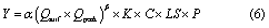
where Y is daily sediment yield (tons), Qsurf is surface runoff (m3), Qpeak is peak runoff rate (m3 s−1), K is the soil erodibility factor, C is the cover and management factor, LS is the topographic factor, and P is the support practice factor. K, C, LS, and P are all unitless factors ranging from 0–1 The coefficient and power constants for the MUSLE, given as 11.8 and 0.56 respectively for metric units in Williams (1975), are location-specific parameters that are often calibrated (Sadeghi et al 2014). Motew et al (2017) calibrated these parameters to be 5.9 and 0.35, respectively.
The calculation for sediment P (SP) is made in units of kg ha−1 using the following equation:
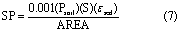
where Psoil is the concentration of sediment P in soil (g P ton−1 soil), S is sediment yield (tons), and εsed is the P enrichment value, defined as the ratio of the concentration of P transported with sediment to the concentration in the surface soil layer (Sharpley 1985). The concentration of sediment P in soil is calculated using the sum of P in all soil pools:
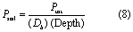
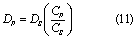
where Ptot is the sum of P in the surface soil layer for the three inorganic pools as well as the two organic pools (kg ha−1), Db is the soil bulk density (g cm−3), and Depth is the depth of the surface soil layer (mm).
Further details regarding the terrestrial P module, including losses of P in runoff and soil P transformations are given in the appendix of Motew et al (2017), available online at www.github.com/mmotew/Appendix-Motew-et-al-2017.git.
A.3. Stream level dissolved and sediment P transport
The in-stream transport of dissolved and sediment P is modeled by THMB. In the modeling framework, dissolved P is considered to be chemically inactive. As a result, dissolved P is simulated as a conservative solute, which follows water flow in stream networks. For sediment P, the in-channel erosion process is modeled using the following equations (Viney et al 2000):
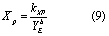
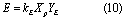
where Xp is in-channel enrichment ratio; XXP is enrichment coefficient; YE is sediment erosion rate (kg s−1); b is enrichment optimization parameter; E is sediment P erosion rate (kg s−1); and kE is sediment P erosion coefficient. In-channel sediment P deposition is assumed to be proportional to sediment deposition, which is quantified using the following equation:
where DP is sediment P deposition rate (kg s−1); DS is sediment deposition rate (kg s−1); CP is sediment P concentration (kg m−3); and CS is sediment concentration (kg m−3). The in-channel sediment P storage is tracked in THMB at each time step and the amount of sediment P erosion will not exceed the storage in each grid cell.
Appendix B. Climate data generation
To generate the climate data, we first created two daily precipitation time series using the rectangular Poisson pulse model (Eagleson 1978). In this model, precipitation is simulated as a series of discrete random storms where storm intensity, storm duration, and inter-storm period are each expressed by an exponential distribution:
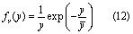
where y is an exponentially distributed random variable with mean . We used (12) to simulate storm intensity (i), storm duration (tr), and inter-storm period (tb). Storm depth (h) is the product of storm intensity and duration, h=i⁎tr. The simulated rainfall time-series was created by randomly drawing from these three distributions to determine i, tr and tb for the subsequent precipitation event, under the assumption that i, tr and tb were independent. To represent seasonality of precipitation, the parameter of each function was varied on a monthly basis using data from Hawk and Eagleson (1992) for La Crosse, Wisconsin. To generate two time-series with highly diverging precipitation regimes, we adjusted the initial monthly parameters for mean storm intensity and inter-storm period using a multiplier (table 1). The HI regime had multipliers greater than 1 indicating a higher mean storm intensity and longer inter-storm period, while the LO regime had multipliers less than 1. The differing parameter multipliers were adjusted to meet the requirement that mean annual precipitation be nearly identical in both regimes (table 1). The LO regime was similar to the current climate in terms of the 99th percentile daily precipitation rate and the HI regime was similar to the more extreme CMIP3 climate projections for the region (Notaro et al 2014) (table 1). Once generated, the hourly storm events were tabulated into daily precipitation amounts to be input to Agro-IBIS. To support model performance of streamflow in THMB, as determined through prior calibration (Motew et al 2017), daily precipitation amounts in Agro-IBIS were distributed evenly over an 8 hr storm period. While this may have caused a loss of detail in daily storm characteristics, the imposed 8 hr storm length was applied to both precipitation regimes and was therefore not expected to interfere with the underlying differences between HI and LO.
Maximum and minimum daily air temperature (Tmax and Tmin) were generated using a method similar to that in the WGEN stochastic weather simulation model (Richardson and Wright 1984). Mean and standard deviation of Tmax and Tmin were determined for each day of the year for the Madison climate record (1996−2015), conditioned on wet and dry days. A Fourier model was then fit for all eight statistics. A daily residual was calculated using a weakly stationary generating process that preserves serial- and cross-correlation and adds a stochastic component. Daily Tmax and Tmin were then calculated based on modeled mean and standard deviation and whether the day is wet or dry. The remaining climate variables were estimated using regression models with a stochastic component presented in Booth et al (2016).
Appendix C. Data analysis
Annual average watershed values of P quantities, including yield, concentration, and load, were examined for an interaction between PSUP and PREC. We used two-way ANOVA for a 2 × 2 factorial design to test the interaction effect of these drivers, treating both as categorical variables. An interaction between PREC and PSUP was statistically significant if the p-value for the interaction term was less than 0.05. P loss from specific sources of P including soil, fertilizer, and manure, were tested separately for an interaction with precipitation intensity. This was done because losses of P from soil, fertilizer and manure were calculated independently within the model. Testing the three sources individually for interactions helped determine which terrestrial pool of P was responsible for any observed interactions, and suggested the underlying biophysical mechanisms responsible.
We used QQ plots and the Shapiro-Wilk test to check for normality of each P quantity prior to performing ANOVA. If the distribution was not approximately normal, we used log10 transformation and re-tested for normality. Based on this procedure, all P quantities warranted a log10 transformation. However, we also performed ANOVA on the untransformed distributions since in some cases ANOVA revealed a significant interaction in the untransformed data and no significant interaction in the transformed data, indicating a removable interaction (de González and Cox 2007). Identifying removable interactions was helpful in the overall interpretation of results.
For those P quantities that had a significant interaction between PREC and PSUP, we generated interaction plots to visually examine the nature of the interaction, i.e. if they were synergistic, inversely related, etc We also generated plots of probability density for those quantities using the 'ksdensity' kernel smoothing function in MATLAB. For analysis at the field scale, annual P yield was calculated as the sum of daily yield, averaged over all terrestrial grid-cells. For annual P concentration at the field scale, annual yield was divided by total annual runoff volume. A similar approach was taken at the stream scale, where daily loads to Lake Mendota were summed over the year to obtain annual load, and annual concentration was obtained by dividing annual load by total streamflow volume. All annual P variables were calculated for the water year, defined as November 1–October 31. All statistical analyses were performed using the Statistics Toolbox in MATLAB (The MathWorks Inc. 2015).