

Abstract
This review addresses the causes of observed climate variations across the industrial period, from 1750 to present. It focuses on long-term changes, both in response to external forcing and to climate variability in the ocean and atmosphere. A synthesis of results from attribution studies based on palaeoclimatic reconstructions covering the recent few centuries to the 20th century, and instrumental data shows how greenhouse gases began to cause warming since the beginning of industrialization, causing trends that are attributable to greenhouse gases by 1900 in proxy-based temperature reconstructions. Their influence increased over time, dominating recent trends. However, other forcings have caused substantial deviations from this emerging greenhouse warming trend: volcanic eruptions have caused strong cooling following a period of unusually heavy activity, such as in the early 19th century; or warming during periods of low activity, such as in the early-to-mid 20th century. Anthropogenic aerosol forcing most likely masked some global greenhouse warming over the 20th century, especially since the accelerated increase in sulphate aerosol emissions starting around 1950. Based on modelling and attribution studies, aerosol forcing has also influenced regional temperatures, caused long-term changes in monsoons and imprinted on Atlantic variability. Multi-decadal variations in atmospheric modes can also cause long-term climate variability, as apparent for the example of the North Atlantic Oscillation, and have influenced Atlantic ocean variability. Long-term precipitation changes are more difficult to attribute to external forcing due to spatial sparseness of data and noisiness of precipitation changes, but the observed pattern of precipitation response to warming from station data supports climate model simulated changes and with it, predictions. The long-term warming has also led to significant differences in daily variability as, for example, visible in long European station data. Extreme events over the historical record provide valuable samples of possible extreme events and their mechanisms.
Export citation and abstract BibTeX RIS

Original content from this work may be used under the terms of the Creative Commons Attribution 3.0 licence. Any further distribution of this work must maintain attribution to the author(s) and the title of the work, journal citation and DOI.
1. Introduction
Much of the research on climate change and climate variability has focused on analyses of the second half of the 20th century. This is highlighted by the conclusion of the 5th Assessment Report (AR5) of the Intergovernmental Panel on Climate Change (IPCC) that 'it is extremely likely that more than half of the observed increase in global average surface temperature from 1951 to 2010 was caused by the anthropogenic increase in greenhouse gas concentrations and other anthropogenic forcings together' (Bindoff et al 2014). That statement was supported by analyses using the full instrumental time horizon, but results are clearer and uncertainties better understood when focusing on the past 60 years (see e.g. Gillett et al 2012, Jones et al 2013). However, some analyses focus on the entire historical record or a large fraction of it, starting with Hulme and Jones (1994) and Andronova and Schlesinger (2000), and multiple analyses of the instrumental period are available. The IPCC report on 1.5 degrees of warming concluded, based on multiple attribution analyses, that 'Estimated anthropogenic global warming matches the level of observed warming to within ±20% (likely range)' (IPCC 2018).
Much of the analysis of extreme events also focuses on recent events, including attributing causes to extreme events soon after they occurred (Stott et al 2016, 2018), but the historical and early instrumental record contains a wealth of information on past events that if used with caution can provide valuable samples of possible events. Also, while decadal prediction tools are tested on hindcasts of the recent past, some analyses suggest decadal changes in predictability and hence biased results when limiting hindcasts to only a few decades (O'Reilly et al 2017, Weisheimer et al 2017), again emphasising the benefit of using the full record.
Focusing on the recent past has clear advantages: observational data are much more complete and reliable, particularly over the satellite period when global or near-global coverage emerged. In contrast, early instrumental data show increasing gaps further back in time (Morice et al 2012), and are affected by uncertainty due to changing sea surface temperature (SST) measurement practices (Thompson et al 2008, Kennedy et al 2011a, 2011b, Morice et al 2012, Kent et al 2016). However, a longer time horizon better constrains the response to forcing (Gillett et al 2012, Jones et al 2013), and reduces spurious correlation between forcings that can yield degenerate results. A longer time horizon also provides a better sample of internal climate variability, particularly of decadal modes. This is important as a short sample can make it harder to tease apart the contribution of variability generated within the climate system and that occurring in response to forcing, for example, in the case of the Atlantic Multidecadal Variability (AMV; e.g. Knight 2009, Ting et al 2009, Booth et al 2012, Tandon and Kushner 2015, Undorf et al 2018a). Lastly, analyses of the instrumental period and the last millennium overlap with some long instrumental records stretching back into the 17th century (Manley 1974, Rousseau 2015). Estimates of global temperature based on palaeoclimatic data are spatially sparse, but more evenly spaced across the globe (e.g. Crowley et al 2014). Some regional reconstructions successfully use a combination of long historical records with proxy information (Luterbacher et al 2004), yet the most recent results attributing fluctuations to external forcing are based on analysis of either instrumental data or proxy-based reconstructions (e.g. PAGES 2k Consortium et al 2013), and the results have not been brought together in a coherent framework.
Here we discuss causes of climate change and estimates of climate variability over a longer time horizon, stretching over the length of the instrumental global data into the 19th century; and linking results to those from analyses of the last millennium. For precipitation, we focus on changes over the 20th century due to the sparsity of earlier records and the need for better sampling to record spatially inhomogeneous changes. We also discuss the contribution to multidecadal trends by variability generated within the climate system, both in the atmosphere and ocean. For the latter topic we focus on the Atlantic Sector due to better coverage back in time. Specifically, we address the following questions:
- When did the response to greenhouse gases emerge on hemispheric and global scales?
- What factors cause decadal and multidecadal deviations from the greenhouse warming trend?
The paper briefly discusses methods and data, followed by a review of causes of climate change over the industrial period (section 3), a brief review of causes and consequences of multidecadal climate variability (section 4), and of related extremes (section 5) and draws some conclusions and recommendations.
2. Data and methods
Data sources become sparser and their quality worse back in time, with observations largely limited to the surface of the Earth. Gridded global instrumental surface temperature data sets (Jones et al 2012, Morice et al 2012) presently stretch to 1850, with estimates of uncertainty available that include both the effect of sampling uncertainty and systematic changes in measurement techniques, such as different types of buckets (Folland and Parker 1995). While the record is fairly well researched, issues continue to be discovered, such as an inhomogeneity in SST data in the 1940s (Thompson et al 2008); and ongoing offsets due to differences in observing fleets (Chan and Huybers 2019). Long, homogenized instrumental surface temperature records go back to the 18th century for some European locations such as Milan, Stockholm, and Central England, resolving daily variability (e.g. Parker et al 1992, Maugeri et al 2002, Moberg et al 2002), while the US Global Historical Climatology Network dataset also contains a limited number of long daily recordings (see e.g. Kenyon and Hegerl 2008). Homogeneity can be an issue for long stations. For example, there is a hot bias for sunny days due to the lack of shielding of summer temperature measurements before the invention of the Stevenson screen in 1864 (Stevenson 1864, Böhm et al 2010, Naylor 2019). There is considerable scope to extend the instrumental record back in time, using long stations and undigitized records (e.g. Brönnimann et al 2019b).
Long-term gridded precipitation datasets (Zhang et al 2007, Becker et al 2013, Harris et al 2014) are sparse, particularly prior to the middle of the 20th century. Reconstructions are available for past hemispheric and continental-scale temperature and to a lesser extent also for drought (e.g. Luterbacher et al 2004, PAGES 2k Consortium et al 2013, Anchukaitis et al 2017, Steiger et al 2018). Also, sea ice data from the early 20th century are being increasingly digitised, allowing better reflection, for example, of the early 20th century sea ice retreat in data (Titchner and Rayner 2014, Walsh et al 2017, Hegerl et al 2018).
Global coverage of the 3D atmosphere is available from historical reanalyses that assimilate surface and sea level pressure and, in some products, marine winds (Compo et al 2011, Poli et al 2016, Laloyaux et al 2018). These provide a dynamically consistent estimate of the atmospheric state from 1851 to 2008, with updates in preparation going back further. Changes in data support can introduce inhomogeneities in reanalyses over time, hence trends have to be treated with caution (e.g. Ferguson and Villarini 2012, Krueger et al 2012). Inhomogeneities are less of a concern where analysis is constrained to the response to well observed modes of climate variability or to episodic forcing such as volcanic eruptions. Hence, with caution, the reanalyses can inform on causes and dynamical links of past anomalies. Reanalyses are now being pushed back into the early industrial period which, for example, has allowed an estimate of the large-scale anomalies following the eruption of Mount Tambora in 1815 (Brohan et al 2016). Data assimilation techniques are also used to obtain 3D reconstructions further back in time (e.g. Franke et al 2017, Tardif et al 2019).
Using early records in analysis of mechanisms as well as detection and attribution requires careful treatment of missing values and consideration of data coverage, usually limiting the analysis to data-covered areas in both observations and climate models. This avoids, at least to some extent, introducing biases due to uneven distribution of data across the globe (e.g. limited coverage in high latitudes, Cowtan et al 2015); and also circumvents relying on assumptions made in infilled datasets. Estimates of data uncertainty are important in order to evaluate how they translate into the uncertainty of specific findings based on these data (Morice et al 2012).
Some of the results presented here rely on widely used detection and attribution methods. These have been recently reviewed (e.g. in Bindoff et al 2014) and are only briefly outlined here. The regression-based detection and attribution method used here assumes that an observed climate change y is regarded as a linear combination of externally forced signals X and residual internal climate variability u, where X is an m × n matrix with each of the m columns a separate fingerprint of dimension n, that captures the expected time-space pattern of change in response to a combination of m individual forcings. These include typically greenhouse gases, other anthropogenic factors (such as aerosols) and natural forcing (Xi, i = 1..m = 3) (e.g. Hasselmann 1997, Ribes et al 2013):

This equation assumes that forcings superimpose linearly. Linearity has been queried, and does not apply while under radiative imbalance (Goodwin 2018). Also, feedbacks can change with the climate state. On the other hand, the nonlinear effect of radiative imbalance over the historical period should be small outside the immediate aftermath of strong eruptions; and swamped by large climate variability. Consistently, linearity has been found appropriate for large-scale changes in temperature across the historical period (Shiogama et al 2013) and, along with a large body of work, we assume it here. y represents the observed record, usually after distilling it into a small-dimensional space n. This can be done by truncating to a limited number of Empirical Orthogonal Functions (Hegerl et al 1996, Hasselmann 1997, Tett et al 1999) or using only few spatial indicators such as global mean temperature, hemispheric contrast and summer/winter contrast (Schurer et al 2018). The outcome of the analysis is a vector of m scaling factors a that adjusts the amplitudes of each fingerprint to best match observations.
Fingerprints are usually derived from coupled climate model simulations, often by averaging across simulations from multiple models in order to both reduce noise from internal climate variability and to average across model uncertainty (the multi-model mean). Uncertainties in a are estimated by accounting for the effect of climate variability on y, usually using samples from climate model control simulations. When the uncertainty range around a fingerprint's scaling factor ai is statistically separated from zero, the fingerprint i is detectable, and where it is significantly smaller or larger than '1' the best-guess response in observations is significantly smaller or larger than in the models. X may contain noise if, for example, it arises from averaging across a limited number of climate model simulations. In this case a total least square regression may be applied (Allen and Stott 2003), which also accounts for noise in X in the calculation of a and its uncertainty. Also, different climate models may simulate a different response to forcing leading to uncertainty in X which can lead to uncertainty not captured in standard methods (Hannart et al 2014, Schurer et al 2018). The latter study found that the widespread practice of inflating (in the specific case, by a factor of 2.6) the climate model variance approximately removes overconfidence in results for large-scale temperature, and so we apply it here for simplicity.
Process studies from climate model simulations can provide powerful evidence for how forcing may have influenced climate, even if links cannot be demonstrated in observations based on detection and attribution, for example, in regions of low signal-to-noise ratio. In section 3 we show some results for the likely contribution of aerosols to regional climate based on modelling.
Another important cause of climatic fluctuations is variability generated within the climate system, either by atmospheric or ocean dynamics, or their interaction. Detection and attribution work considers this variability generally as 'noise'. However, some approaches quantify the effect of modes of variability directly, as is done for example using the Cold Ocean Warm Land pattern (Wallace et al 1995). In the present paper we give some examples showing how decadal or multidecadal temperature fluctuations can arise from (probably) random long-term tendencies in the North Atlantic Oscillation (NAO) and the ocean response to it.
3. Role of forcings in large-scale climate change over the instrumental period
3.1. Observed and simulated global-scale changes in temperature
The 19th century began as one of the coldest periods of the last millennium, at least for the Northern Hemisphere (see Masson-Delmotte et al 2013), following a slightly warmer 18th century (figure 1). Some of the coldest observed periods followed in the two years after the powerful eruption of Mount Tambora in 1815 (Raible et al 2016). After that, temperatures began to show a slow rise, interrupted by cooling induced by volcanic eruptions in the 1830s (Brönnimann et al 2019a) and then the Krakatoa eruption in 1883 (see figure 1). Global temperatures rose particularly rapidly over the early 20th century, showing anomalous warming from the 1920s through the 1940s (see figure 1; and Hegerl et al 2018), before plateauing in the 1950s and 60s, and beginning their strong ongoing increase.
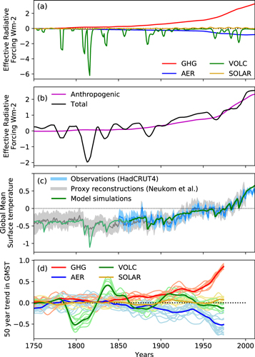
Figure 1. External forcing compared to observed global temperature data. (a) Radiative forcing over the industrial period from IPCC AR5 (Myhre et al 2013) for individual forcings (smoothed by a 3 year running mean), and (b) decadally smoothed (11 year running mean, followed by a 7 year running mean; natural forcings centred on long-term average, 1750–2011) anthropogenic and combined forcing over the industrial period. (c) Observed (Morice et al 2012) and reconstructed global temperature anomalies ([K], Neukom et al 2019), as well as multi-model mean simulations which are generated by merging 23 last millennium simulations from 7 models: bcc-csm1-1(×1), CCSM4(×1), CESM1(×10), CSIRO-Mk3l(×3), GISS-E2-R(×3), HadCM3(×4), MPI-ESM-P(×1) with 109 CMIP5 historical simulations from 41 models (see methods), anomalies calculated from a 1961–1990 climatology. (d) Running 50 year trends (trend calculated from timeseries smoothed by a 5 then 3 year running average, plotted against central time point, [K/50 yrs]) that illustrate trends caused by individual forcings in two models (HadCM3 and CESM1) (thicker lines: multi-model mean, thinner lines: individual simulations).
Download figure:
Standard image High-resolution imageMuch of this temperature variability has been driven by external forcing (figure 1): following a small dip of CO2 in the Little Ice Age (Schmidt et al 2012, Masson-Delmotte et al 2013), CO2 began to rise since the beginning of industrialization along with other greenhouse gases. The strongest increase in radiative forcing by greenhouse gases occurred in the recent few decades, an increase that is steadily continuing to date. With the burning of fossil fuels, anthropogenic aerosols began to increase as well, with aerosol forcing estimates peaking globally around 1980, although emissions have continued increasing in South and East Asia while decreasing in Europe and North America since then.
Natural forcing has imposed decadal scale variations on the total forcing (figure 1): while global radiative forcing by solar irradiance variations was quite small, with an increase towards the mid-20th century and a minimum in the 17th and early 19th centuries, episodic volcanic eruptions caused periods of stronger or weaker than average negative forcing. The largest was the eruption of Mount Tambora in 1815, which came shortly after an eruption of unknown origin in 1808 or 1809 (Guevara-Murua et al 2014, Cole-Dai et al 2016, Raible et al 2016). A strongly smoothed version of the total forcing (anthropogenic and natural forcings combined) deviates from the anthropogenic forcing substantially over some periods, most notably, the period around the Tambora eruption, and the mid-20th century. The natural forcing in the latter period is largely due to a hiatus in volcanism. It has been argued that volcanic eruptions only cause short-term cooling. However, climate model simulations show an extended cold period following the 1809/Tambora period, with no single year in model simulations with HadCM3, for example, reaching the average of the 20 years prior to the eruptions up to the 1830s (Schurer et al 2014), when another period of volcanism kept temperature low until the 1840s (Brönnimann et al 2019a). Equally, climate models simulate long-term warming in periods with little volcanic forcing, such as the early 20th century (Hegerl et al 2018). The climate model simulated response to all forcings combined (multimodel mean, concatenated between Coupled Model Intercomparison Project Phase 5 (CMIP5) and Paleoclimate Modelling Intercomparison Project (PMIP) simulations, see methods; figure 1(c)) closely follows the forcing and replicates the observed and reconstructed global temperature estimates largely within uncertainties. Some studies have argued that the response to forcing could account for more of the observed global variability if forcing uncertainty is taken into consideration (Haustein et al 2019).
The observations deviate from the model mean and range during some periods, the first of which is 1900–1910. This was a period of anomalously cold SST conditions developing in the South Atlantic and spreading northward (Hegerl et al 2018). Both long-term homogeneous stations in southern Africa and South America as well as ship data support the anomalously cold conditions during this period, which clearly deserves more attention (see discussion of ocean below). Observations are warmer than models during the peak of the early 20th century warming around 1940, which was particularly pronounced in the Arctic and Atlantic sector (Brönnimann 2009, Wood and Overland 2010, Hegerl et al 2018). The most recent deviation between climate models and observations occurred during the 'hiatus' of warming from around 1998 to 2012 (figure 1(c); Lewandowsky et al 2016, Yan et al 2016, Medhaug et al 2017) which has since ended with global warming rapidly resuming (Hu and Fedorov 2017).
The spatial pattern of observed trends (figure 2) shows that both warming and cooling/flat periods can show distinctly different spatial signatures. A trend towards cool conditions in some regions prior to 1910 shows also relatively cool conditions in data covered parts of the Southern Ocean. The early 20th century warming emerges from this cold period (figure 2(b)), which is equally strong or stronger over ocean and, while it started with strong Arctic and North Atlantic warming (Hegerl et al 2018), it is relatively uniform for the 1910–1950 trend. From 1950 to 1980, observations show a hemispherically asymmetric spatial trend pattern, with more regions warming in the Southern Hemisphere and some oceanic regions of cooling in the Northern Hemisphere (figure 2(c)). From 1980 onwards, a strong warming emerges that is almost global in nature with very strong trends (figure 2(d)). Exceptions are the off-equatorial and tropical regions of the central and eastern Pacific associated with the transition to a negative Interdecadal Pacific Oscillation phase (Zhang et al 1997, Power et al 1999) coincident with the early-2000s hiatus (Kosaka and Xie 2013, England et al 2014), and the high-latitude Southern Ocean (Armour et al 2016, Jones et al 2016).
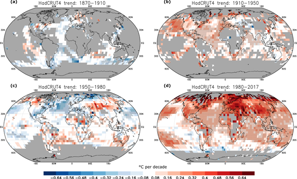
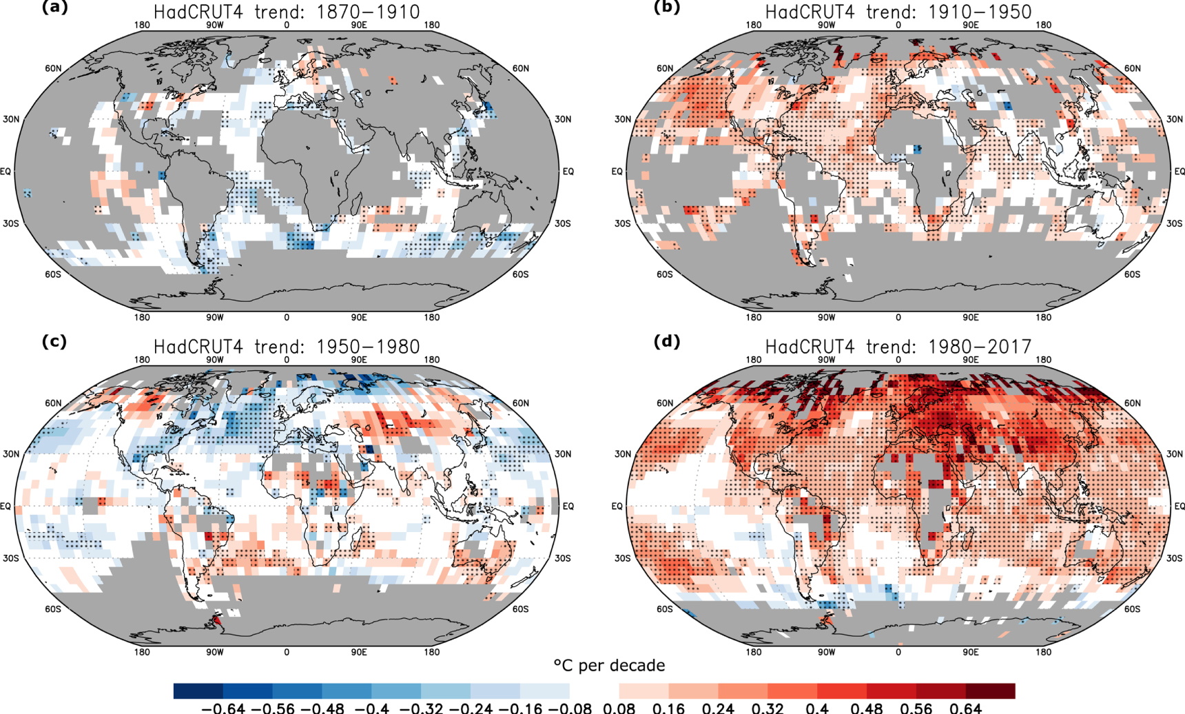
Figure 2. Long-term multi-year trends over the instrumental period [°C per decade]. HadCRUT4 (Morice et al 2012) 3 year running mean annual mean (November–October) trends over: (a) 1870–1910, (b) 1910–1950, (c) 1950–1980, and (d) 1980–2017. The 3 year annual means are constructed from averaging November–April and May–October anomalies, each smoothed with a 3 year running mean. Grey areas indicate regions where each overlapping 3 year segment does not contain at least one datapoint from both November–April and May–October. The slopes are stippled where significant at p < 0.05 using a 2-tailed t-test, adjusted for autocorrelation induced by the 3 year running mean by increasing the regression standard error by a factor of  and by using 1 degree of freedom for every 3 years of length.
Download figure:
Standard image High-resolution image3.2. Causes of global-scale changes in temperature
What caused these spatially diverse long-term trends? The similarity between simulated and observed/reconstructed changes in figure 1 suggests a strong role of external forcing. Detection and attribution methods are able to disentangle which of the forcings have played key roles in observed changes, and which are less important. Table 1 summarizes published global and hemispheric scale detection and attribution results from various timelines. Analysis of palaeoclimatic records for hemispheric and global mean data suggests that significant trends in response to greenhouse gas increases can already be detected and attributed by 1900, both across the Northern Hemisphere and in some regions such as Europe (Hegerl et al 2011, PAGES 2k Consortium et al 2013, Schurer et al 2014). This result is based on an analysis that captures the time evolution of hemispherically averaged temperature from the 15th century (table 1) and hence captures both the temperature response to a sustained, small CO2 drop over parts of the Little Ice Age (Koch et al 2019) and the response to the CO2 increase following industrialization. Abram et al (2016) also found sustained warming in regional proxy-reconstructions from the early mid-19th century, consistent with climate modelling.
Table 1. Example of detection and attribution results from the literature, starting from the last millennium (top) to instrumentally based (bottom). A detectable response in greenhouse gases is indicated by Y (at either the 5 or 10% significance level), and 'consistent' refers to a scaling factor encompassing '1', i.e. the average of the combination of models used not needing to be rescaled to match observations. For analyses which have analysed individual models separately we give the fraction of models in which the forcing is detectable. Nat refers to natural forcing, OANT to anthropogenic forcing other than greenhouse gases, ANT to anthropogenic forcing combined. MM refers to the multi model mean.
| Paper | Period/Exp | Models | Detection of greenhouse gas influence | Detection of other forcings |
|---|---|---|---|---|
| PAGES 2k Consortium et al (2013), PAGES 2k-PMIP3 group (2015) | 864–1840 | PMIP3 | Not attempted | All forcings detectable in NH continents but not SH |
| 1013–1989 | ||||
| 1350–1840 | ||||
| Schurer et al (2013) | 1400–1900, NH; reconstructions | PMIP | Y (most reconstructions, consistent) | Nat generally detectable and consistent, best guess <1 |
| Schurer et al (2014) | 1450–1900 NH multi-reconst. | HadCM3 | Y | Volc detectable, solar consistent but not significant |
| Hegerl et al (2011) | 1500–1996, Europe only; proxy + instrumental | 3 last millennium simulations | ANT ∼ det. in winter and spring | volc. Detectable in EPOCH analysis, solar not robustly detectable |
| Schurer et al (2018) | 1862–2012 instrumental | CMIP5 individual models | Y (consistent) | OANT close to detection; NAT detectable, ∼0.7 but consistent |
| Jones et al (2013) | 1901–2010 | CMIP5 individual models | Y 8/16 cases | Nat detectable 8/16 |
| 1906–2005 instrumental | Y 8/15 and MM mean | Nat detectable 8/15 and MM mean ; both: OANT mostly not detectable in indiidual.models | ||
| Jones and Kennedy (2017) | 1906–2005 instrumental with uncertainty | CMIP5 MM | Y small uncertainty | All others combined D |
| Gillett et al (2013) | 1861–2010 | CMIP5 and individual models | Y 7/9 and | Nat detectable in 7/9 and MMM with model uncertainty |
| MM mean including model uncertainty | OANT detectable in 5/9 cases and MMM only when not including model uncertainty | |||
| Ribes and Terray (2013) | 1901–2010 | CMIP5 and individual models | Y 4/10 | Nat detectable in 4/10 and OANT detectable in 1/10 cases |
However, volcanism is important over much of the 19th century as well: figure 1(d) illustrates that in models, the warming period up to the eruption of Krakatoa was in large parts a relaxation from a period of heavy volcanism around the Mount Tambora eruption (Brönnimann et al 2019a). From the 50 year trend centred around 1860 onwards (ending around 1885, figure 1(d)), climate models indicate that the warming trend originating from the recovery after heavy volcanism is exceeded by the warming trend caused by greenhouse gas increases. Detection and attribution analyses (table 1) confirm detectable responses to both forcings.
Analyses over the entire instrumental period robustly detect the influence of greenhouse gases when using fingerprints that are derived by averaging across many available climate models. Results based on fingerprints from individual models can vary more, with separate detection of greenhouse gas responses in an analysis simultaneously estimating natural, greenhouse gas and aerosol forcing only in about half of the models (Gillett et al 2013, Jones et al 2013, Ribes and Terray 2013). However, integrating attribution results across model uncertainty in a Bayesian analysis yields a robustly detectable greenhouse gas signal even in the presence of model uncertainty (Schurer et al 2018). The response to other anthropogenic forcings, particularly from aerosols, is less clearly detectable unless prior assumptions exclude very large or negative responses (Schurer et al 2018) and their role in regional anomalies is discussed below (see also table 1; Bindoff et al 2014).
Both for reconstructed palaeoclimate and climate over the instrumental period, the response to natural forcing (solar and volcanic combined) is robust across studies, although the best estimate magnitude is only about 70% of that in climate model simulations (see also figure 3). Scaling factors in the top panel indicate the best fit and uncertainty range of the magnitude of the model simulated pattern to observations a in equation (1). In instrumental data this slightly smaller response to natural forcing may, at least in part, be due to the confounding effect of El Niño events in the later 20th century following eruptions which, when accounted for, brings models and observations in closer agreement in attribution studies (Lehner et al 2016). A strong role for volcanism in decadal temperature variability is confirmed in detection and attribution studies for the last millennium (table 1; see Bindoff et al 2014, Schurer et al 2014) although again the amplitude of detected changes appears smaller in reconstructions than model simulations. Volcanism has also been implicated in long-term hiatus and surge events of global warming (Schurer et al 2015, Neukom et al 2019).
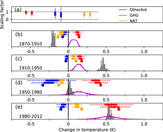
Figure 3. Estimated contribution by forcing to observed changes across the instrumental record. This is based on HadCRUT4 surface temperature data with histograms reflecting uncertainty (Morice et al 2012). (a) Estimated magnitude of the response to forcing by greenhouse gases (GHG, red), other anthropogenic forcing (OtherAnt, blue) and natural forcing (solar and volcanic, NAT, yellow). Results are based on a Bayesian approach over the full period (1863–2012) using the multimodel mean response (Schurer et al 2018); using global mean and hemispheric difference as spatial components, and decadally averaged timeseries. Values in the bottom four panels are calculated by scaling the linear trend by the best fit of the model fingerprint to observations over the entire record. The purple line is the combined anthropogenic contribution to the change in that period, the grey histogram is the range of observational values. The thick line indicates the 33–66th percentile, the thin line 5%–95% of the uncertainty, and the continuous line is an estimate using prior information that favours scaling near one and avoids unphysical negative scaling, while the dashed line shows results for a flat prior between −1 and 3. Circles in each of the bottom panels indicate the multi-model mean estimate of the forced contribution without scaling. Note that the prior information makes little difference to the estimate of the total anthropogenic contribution, but does affect the estimate of individual forcings.
Download figure:
Standard image High-resolution imageOnly few studies are available that estimate the role of solar forcing alone. Over the last five centuries, reconstructions support only a moderate magnitude of solar forcing (Schurer et al 2014), as do analyses of the instrumental period based on formal attribution (Stott et al 2003, Benestad and Schmidt 2009) and global time series regression analyses (Folland et al 2018, Lean 2018). Analysis also suggests a role of solar forcing in trends (figure 1(d)), although it is not significant against internal variability in climate models (indicated by the spread of simulations) yet may have slightly influenced trends. The solar influence may be stronger on regional climate where solar forcing may influence modes of climate variability. For instance, during solar minima, there appears to be an increased likelihood of the negative phase of the NAO and increased North Atlantic/Eurasian blocking frequency (Lockwood et al 2010), linked with cold winters in Europe and warm ones in Greenland (e.g. Woollings et al 2010, Ineson et al 2011, Scaife et al 2013, Gray et al 2016). Possible effects have also been found on equatorial Pacific SSTs, sea level pressure in the Gulf of Alaska and the South Pacific, the strength and location of tropical convergence zones, the strength of the Indian monsoon and the location of the descending branch of the Walker circulation, impacting on precipitation (Meehl et al 2009, Gray et al 2010, Bindoff et al 2014, and references therein). These hypothesized effects may either arise through SST influences, or through solar influence on the stratosphere (Gray et al 2010), and remain uncertain.
Figure 3 shows the implications of detection and attribution of greenhouse gas, other anthropogenic, and natural forcings over the instrumental period on causes of the trends over the periods shown in figure 2 (note that the results shown are from Schurer et al (2018) but are qualitatively and quantitatively similar to those in other studies, table 1). The attribution analysis is based on a multimodel mean fingerprint over the instrumental period, with uncertainties enlarged to avoid overconfidence (by increasing the variance of the control simulation by a factor of 2.6, see methods and Schurer et al 2018). It yields a well-constrained greenhouse gas response that is consistent and close in magnitude to the multi-model mean response in climate models. It also shows a detectable response to natural forcing, which is slightly smaller in observations than in climate models (figure 1, yellow). The response to other anthropogenic forcing is more uncertain and depends on prior assumptions (figure 3(a), the informative prior assumes no negative scaling factors and decay at about 3, peaking at 1 while the flat noninformative prior covers a −1 to +3 range).
These attribution results can be interpreted as observation-based estimates of the contribution of forcing to different periods, in a similar way that the IPCC has estimated the greenhouse gas contribution to the recent 60 years (Bindoff et al 2014). This is done by inflating or deflating the multi-model mean forced contribution to a period within the range of the estimated scaling factors. Note that interpreting the results of the long analysis over shorter segments carries additional uncertainties in that errors in the time evolution of the response may impact shorter periods, yet average out over longer periods. Where this occurs, uncertainties over the shorter period may be larger than indicated by the scaling factor uncertainty only.
Results show that the observed cooling from 1870 to 1910 in observations (uncertainty in observed change expressed in grey histogram, Morice et al 2012) occurred despite a small greenhouse forced warming, and appears to be due to a combination of internal climate variability, natural forcing (e.g. Mount Krakatoa eruption) and aerosols. The noticeable contribution by greenhouse gases is consistent with the early detection of greenhouse warming from proxy-based data discussed above. This period shows stronger cooling than simulated, consistent with the above discussed period of anomalously cold SSTs in the very early 20th century. The subsequent period (figure 3(c)) is dominated by the early 20th century global warming trend. The combined response to anthropogenic forcing (purple) is smaller than the observed trend, indicating a role of internal climate variability in the warming to 1950 (see also Hegerl et al 2018). The detection and attribution results further suggests that the plateau in observed trends from 1950 to 1980 occurred despite a net positive anthropogenic forcing, which is a strong greenhouse warming counteracted in large part by very strong aerosol induced trends. The analysis indicates that this net anthropogenic forcing was counteracted by slightly negative natural forcing (e.g. eruption of Mount Agung). Subsequently, greenhouse gases caused a strong warming trend from 1980 to 2012 (when CMIP5 simulations end); with the aerosol influence weakening and largely counteracted (in best estimate) by a slightly positive response to natural forcing, which is consistent with the eruption of El Chichon in 1982, and Mount Pinatubo in 1991 in the first half of the period (see also figure 1(d)).
These results, particularly, the varying contribution of natural forcings to different decades across the industrial periods as well as the early detectable greenhouse gas influence illustrates the difficulty of finding a suitable and 'typical' pre-industrial period (Hawkins et al 2017, Schurer et al 2017): periods are influenced differently by natural forcing, and CO2 has been rising since 1750, following its enigmatic drop (Koch et al 2019) around the Little Ice Age. Therefore there is no constant and unambiguous preindustrial background temperature. Figure 1 shows that the period 1850–1900 (which is frequently used as proxy for the pre-industrial baseline due to the availability of instrumental observations with some global-scale coverage; Allen et al 2018) is a fairly stable climatic period with only small trends superimposed on the anthropogenic forcing, which, however, by that time had already caused a warming trend.
3.3. The role of anthropogenic aerosols in regional changes
Model simulations and attribution results suggest that aerosols have been playing a key role in shaping regional climate, over the entire 20th century and before. It has been argued that small aerosol perturbations in early industrial time may have caused substantial impacts in a less polluted atmosphere (e.g. Carslaw et al 2013)—with potential consequences for our best estimate of aerosol radiative forcing (Stevens 2015, Kretzschmar et al 2017, Booth et al 2018). This is, however, difficult to quantify as the natural aerosol loading due to biomass burning and natural sources is uncertain, as is the magnitude of aerosol-cloud interactions and therefore the realistic nature of their representation in models (e.g. Zelinka et al 2014, Wilcox et al 2015, Toll et al 2017).
Long-term aerosol impacts on regional climate are supported by climate modelling (figure 4). European mean surface temperature, similar to global temperature, shows a plateau in warming at the period of strongest European and North American aerosol emissions that is reflected in aerosol only simulations, but not in greenhouse gas or natural only runs (figure 4(a)). Furthermore, the observed daily temperature range over Europe has decreased throughout that time period, although with quite strong variability and data uncertainty. Comparison with surface solar radiation (e.g. Wild et al 2007, Makowski et al 2008), and single-forcing simulations (figure 4(b), Undorf et al 2018b) suggest a contribution from anthropogenic aerosols to this decrease. While the temperature impact of aerosols is expected to have been largest over their emission regions, and downstream thereof (e.g. Shindell et al 2010), the global, heterogeneous patterns of temperature change simulated by models (e.g. Shindell et al 2015, Wang et al 2016) suggest relevant impact elsewhere, too. Aerosol impact on other variables is mediated by the change in temperature, as suggested for Arctic sea ice (e.g. Acosta Navarro et al 2016, Mueller et al 2018), or by temperature gradients, like for the inter-tropical convergence zone (ITCZ, Chang et al 2011, Hwang et al 2013, Undorf et al 2018c; see also figures 8(a), (b)) and the strength and position of the Northern Hemisphere subtropical jet stream and the tropical belt width (e.g. Allen and Ajoku 2016, Undorf et al 2018b).
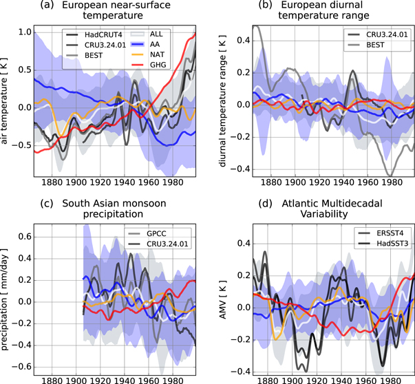
Figure 4. Aerosol influences on European climate, South Asian monsoon and Atlantic Multidecadal Variability. Anomalies of (a)annual-mean near-surface temperature and diurnal temperature range, (b) over Europe (35°–65°N,15°W-30°E, land only, area-weighted) similar to Undorf et al (2018b), (c) summer (JJAS)-mean monsoon precipitation over South Asia (area definition as in Undorf et al 2018c), and (d) the annual Atlantic Multidecadal Variability (AMV) index for (black, grays) observations and simulations with (red) greenhouse gas (GHG) forcing, (blue) anthropogenic aerosol (AA), and (yellow) natural (NAT) forcing only, and (white) all forcings together (ALL). Shown are the ensemble means (lines) and the 1.66σ range (shading) of each multi-model ensemble, smoothed by applying (a)–(c) 7-and 5-point and (d) 11-and 7-point filters consecutively. The shadings for GHG and NAT are omitted for clarity. (d) Sea surface temperatures (SSTs) are not available for all models, so surface temperatures over sea areas are used instead and compared with SST observations. The AMV is derived as in Undorf et al (2018a). The models and the respective number of ensemble members used are CanESM2 [×5], CESM1-CAM5 [×1], CSIRO-Mk-3-6-0 [×5], GFDL-CM3 [×3], GISS-E2-R [×5], HadGEM2-ES [×4] (only in (a) and (c)), IPSL-CM5A-LR [×1], and NorESM1-M [×1].
Download figure:
Standard image High-resolution imageLong-term variability in the monsoons has also been linked to aerosol forcing, in East Asia (Guo et al 2013, Li et al 2016), South Asia (e.g. Bollasina et al 2011, Guo et al 2015), and Australia (Rotstayn et al 2012, Dey et al 2019) as well as over the Sahel (e.g. Rotstayn and Lohmann 2002, Held et al 2005, Ackerley et al 2011, Dong et al 2014). In particular the decrease between the early to mid-20th century and the 1980s and the subsequent recovery in precipitation over the global land surface (Wilcox et al 2013) and global-scale monsoon precipitation, averaged across Asian, African, and American monsoon regions in the Northern Hemisphere, has been attributed to aerosol forcing (Polson et al 2014). The aerosol influence on monsoon precipitation changes in South Asia (figure 4(c)) was found to be driven by a combination of emissions from North America, Europe and South Asia that are all simulated to weaken the monsoon circulation (Undorf et al 2018c). North American and European aerosols, along with natural forcings, are detectable drivers for African monsoon precipitation, but the model simulated changes over this region appear weak compared to observed changes, a source of concern about both modelling future changes and understanding monsoon variability (Biasutti 2013, Polson et al 2014). The dominant mechanism by which the aerosol impact is mediated, on the other hand, seems to be related to shifts of the ITCZ and is as such a well-studied response to aerosol-induced changes of the interhemispheric temperature gradients (Chang et al 2011, Chiang and Friedman 2012, Hwang et al 2013, Undorf et al 2018c; see also figures 8(a), (b)). Related impacts have been suggested on other large-scale atmospheric circulation features like the strength and position of the Northern Hemisphere subtropical jet stream and the tropical belt width (e.g. Allen and Ajoku 2016, Undorf et al 2018b).
3.4. Changes in global-scale precipitation
Global warming will affect the global water cycle and has probably already done so (IPCC 2013). Diagnostics of atmospheric water content and humidity, while showing clear anthropogenic signals (see Santer et al 2007, Bindoff et al 2014) only go back through the satellite era. There is evidence from the mixed satellite/in situ record that the expected intensification of the hydrological cycle with wet regions getting wetter and dry getting drier is indeed detectable, although only if tracking wet and dry regions with the seasonal cycle and over time (Polson et al 2013, Polson and Hegerl 2017). In situ rainfall stations are able to support a longer time horizon, but are spatially sparse, fairly uncertain and only available over land (Zhang et al 2007, Harris et al 2014). However, over land precipitation is influenced by a complex combination of SSTs, land use influences, land-sea contrast and direct forcing (Greve et al 2014), and future changes over land are hence uncertain and strongly model dependent (IPCC 2013). Furthermore, climate model simulations indicate that over the historical period, precipitation changes over land are moderated by other forcings, particularly shortwave forcings (e.g. Richardson et al 2018). Nevertheless, since the second half of the 20th century, a human induced increase in intense precipitation has been detected, consistent with a moister, warmer atmosphere (Min et al 2011, Zhang et al 2013). Similarly, there is some evidence from in situ data over the second half of the 20th century that the high latitudes are becoming wetter (Min et al 2008) although data uncertainty here is substantial (Hegerl et al 2015). Zonal land precipitation shows a change since the 1920s that is broadly consistent with the expected response to anthropogenic forcing (Zhang et al 2007), although particularly seasonal responses are uncertain and noisy (Sarojini et al 2012, Polson et al 2013). Drought atlases from proxy data and instrumental data support a long-term change in drought frequency with a detectable human influence by the middle of the 20th century (Marvel et al 2019). While it remains to be seen to what extent this reflects precipitation change and to what extent increased evaporation due to warming, it provides powerful evidence that greenhouse gases have influenced aspects of the water cycle early on.
In contrast to changes over land, model-simulated precipitation changes over ocean are fairly robust across models, with a signal of wet regions getting wetter and dry regions getting drier. Many precipitation records over islands go back to the 1920s. While they are too sparse to constrain global precipitation changes, the island stations are able to evaluate the pattern of precipitation change associated with global temperature changes: the so-called precipitation sensitivity diagnoses the precipitation response to warming (for any reason including greenhouse gas induced warming) and is expressed as the change [%] in mean precipitation per degree of global mean warming. It has also been found to be a useful constraint on future changes if applied to extremes (O'Gorman 2012). Island stations support a pattern of precipitation sensitivity that is in fairly good agreement with historical simulations from climate models (figure 5) and shows a stronger correlation with historical simulations over the period since 1930 than with satellite data over the period since 1979 (Polson et al 2016). This both supports the simulated large-scale precipitation response and emphasizes the need for long records for noisy precipitation signals. An amplification of the global hydrologic cycle is also supported when using sea surface salinity as an 'indirect rain gauge' (Schmitt 2008, Terray et al 2012): globally from the 1950s (Durack et al 2012, Skliris et al 2014) and over the Atlantic from the early 20th century onwards (Friedman et al 2017).
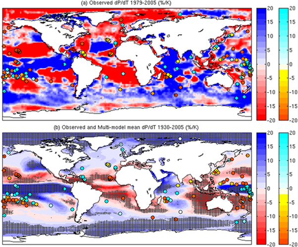
Figure 5. Spatial pattern of precipitation sensitivity (change in precipitation per degree of global mean warming, dP/dT) from satellite/gauge data. (a) Precipitation from the Global Precipitation Climatology Project (GPCP; Huffman et al 2009; from 1979 to 2005) and (b) from multimodel historical simulations 1930–2005 compared to those from long island stations (dots; from CRUTS3.22; Harris et al 2014 in both panels; only small islands used). Figure reproduced from Polson et al (2016), © The Author(s). Published by IOP Publishing Ltd. CC BY 3.0. 65% of gridboxes on top agree on the sign of dP/dT between satellite data and island stations, while 71% of gridboxes agree on the sign of dP/dT between the average dP/dT of individual historical simulations from CMIP5 and island stations. Hatching shows where 75% of CMIP5 simulations agree on the sign of dP/dT.
Download figure:
Standard image High-resolution imageForcing is also expected to directly affect rainfall through a change in energy available for evaporation. Such a response leads, at least in models, to a rapid precipitation decrease after volcanic eruptions over land (Iles et al 2013). The response to greenhouse gas induced warming is muted compared to that to aerosols since changes in lapse rate and atmospheric energy budget constraints reduce the precipitation response to warming (Allen and Ingram 2002, Lambert and Allen 2009, Andrews et al 2010, Bala et al 2010, Cao et al 2012, O'Gorman 2012). This is why the global land response to shortwave forcing such as that from anthropogenic and volcanic aerosols may be more detectable over the historical period than that to greenhouse gas increases (Allen and Ingram 2002). Long-term streamflow data are an excellent opportunity to study the water cycle response to forcing. Several large rivers have streamflow records back into the 19th century. These may reflect changes in response to a combination of precipitation and evaporation, possibly including CO2 induced changes in transpiration (Gedney et al 2006, Piao et al 2007), and can be affected by human influences including irrigation, land use changes, dam construction, and extraction (Gerten et al 2008, Dai et al 2009, Dai 2016). However, they show a detectable and more robustly observed short-term response to volcanic eruptions, with drying on average in the wettest regions of the planet, detectable in the tropics and northern Asia, and detectable wettening in some dry regions such as the southwestern US (Iles and Hegerl 2015).
4. Variability generated within the climate system
In this section we discuss some long-term climate changes that are linked to long-term tendencies in modes of climate variability. It is recognized that external forcing may change the preferred direction and location of modes of climate variability, which is an important uncertainty in future climate change (Shepherd 2014). However, such changes are hard to detect among high circulation variability, hence we only discuss changes caused by trends in circulation, not its causes. At the end of the section, we briefly discuss an example that illustrates why it is difficult to conclude with confidence whether large-scale temperature variability in climate models is consistent with observations.
4.1. Circulation related to atmospheric or coupled variability
Long-term changes in atmospheric circulation are best documented for the Northern Hemisphere Atlantic sector. Here, the NAO is the dominant mode of variability at the surface, and related to variations in storm tracks, particularly, in the winter. The NAO is often defined by the pressure difference between the Icelandic low and the Azores High (e.g. Hurrell 1995), has a distinct spatial pattern of sea level pressure (e.g. Hurrell and Van Loon 1997) and has been observed over a long period of time (Hurrell et al 2003). The NAO is closely related to the Northern Annular Mode (Thompson and Wallace 2001) which is more zonal in nature and links to variations in the polar stratospheric vortex. Due to the longer record, we focus here on the NAO over the Atlantic Sector (Hurrell and Deser 2009). While the NAO is fairly white on timescales longer than interannual, it shows some long-term trends over the period of record. After a variable period with no pronounced trend in the second half of the 19th century, the NAO increased and then showed a marked long-term decrease between the early 20th century and the 1970s. This was followed by a strong upward trend peaking in the 1990s and then a downward trend into the so-called hiatus period (e.g. Hurrell 1995, Thompson and Wallace 2001, les and Hegerl 2017). Winters with an anomalously high NAO index tend to be warmer over Eurasia and anomalously cold in eastern North America and parts of Greenland as well as of the North Atlantic (figure 6, central panel middle). The opposite is true for low NAO values (Hurrell and Van Loon 1997, Iles and Hegerl 2017, figure 6, central panel left and right). If this linear relationship holds for trends in the NAO (and aggregates of NAO trends from climate models suggest it does; Deser et al 2017, Iles and Hegerl 2017) then NAO trends cause long-term temperature changes (figure 6). The NAO decrease to the 1970s may have led to dynamically induced boreal winter trends counteracting greenhouse warming to 1970, then strengthening it to the 1990s, and then counteracting it again. Residual trends, after linearly removing the NAO influence, show a more uniform warming pattern (figure 6 bottom; see also Thompson and Wallace 2001). Not shown is the impact of the NAO on precipitation, which would lead to expected rainfall trends of opposite sign over the Mediterranean and Northwest Europe (Deser et al 2017). Note that based on climate model simulations the ocean response to the NAO trend may enhance the response relative to that estimated from the interannual relationship (see next section; see also Deser et al 2017, Iles and Hegerl 2017 for regression/composite based results).

Figure 6. Influence of North Atlantic Oscillation (NAO) variability on Northern Hemisphere winter temperature trends. Reproduced from Iles and Hegerl (2017) © The Author(s). Published by IOP Publishing Ltd. CC BY 3.0. Top row shows raw observed trend patterns [°C/decade], middle row estimated contribution by the NAO from interannual regression analysis (stippling indicates grid cells with a significant (p < 0.05) interannual relationship between the NAO and temperature), bottom row: trend pattern after linearly removing the contribution by the NAO; note that the residual results for the three periods are far more similar to each other and to the expected pattern in response to anthropogenic forcing than they were initially. Note that oceanic responses to trends in the NAO may enhance the long-term response over the North Atlantic and Arctic ocean basins.
Download figure:
Standard image High-resolution imageThe zonal mean Hadley Circulation is the globally dominant circulation feature, and changes in its location and strength could potentially have large impacts, particularly, on rainfall. Interannual variability in the strength of the Hadley Circulation, as well as its relationship to the El Niño-Southern Oscillation is well studied, but trends in its strength are not well established (Nguyen et al 2012) and reanalyses may show wrong trends (Chemke and Polvani 2019). Nevertheless, a robust widening of the tropical belt is found since ca. 1980 (although reanalyses data sets tend to overpredict the widening; see Davis and Davis 2018). Although climate models predict a widening due to greenhouse gas forcing and also a response to hemispherically heterogeneous aerosol forcing (section 3.3), internal variability is high and yet precludes attribution (Staten et al 2018). The widening from 1980 onward started from a southward shifted state: the northern tropical belt shifted southward from the 1940s to 1980 (Brönnimann et al 2015), and similar decadal changes in the edge of the northern tropical belt have also been found in earlier periods in tree-ring based reconstructions (Alfaro-Sánchez et al 2018).
Furthermore, a weakening of the Pacific Walker circulation was suggested at a centennial scale since the mid-19th century, in line with model simulations (Vecchi et al 2006). However, observations from recent decades point to a strengthening. Apart from data issues, this strengthening might have been due to internal variability, which is a dominant factor controlling the strength of the Pacific Walker circulation (Chung et al 2019). The Walker circulation is closely linked to El Niño, the climate mode with largest global influence, which again shows substantial variability in its variance on multidecadal timescales (Wittenberg 2009). Thus, the contribution of changes in circulation to observed long term changes in precipitation and temperature remains uncertain, as is a possible role of forcing in these changes. This remains a research priority.
4.2. Response and role of ocean and sea ice
The biggest potential source of decadal climate variability is the ocean. Even an inert ocean would cause decadal climate variability by integrating weather noise, and ocean dynamics are expected to enhance this variability (Hasselmann 1976, Frankignoul and Hasselmann 1977). For example, in the GFDL model, a warming episode similar to the early 20th century warming occurred in a historical simulation due to ocean overturning variability (Delworth and Knutson 2000). Figure 7 shows another example based on the Max-Planck Institute ocean model forced by century-long reanalysis ERA20C (Poli et al 2016) with an experimental set up similar to Müller et al (2015). Surface temperatures in the North Atlantic are closely associated with a downward ocean surface heat flux (latent plus sensible heat flux) on an inter-annual timescale (figure 7(b)) and upward into the atmosphere heat flux on decadal to multi-decadal timescales (figure 7(c), see also Gulev et al 2013). This clearly indicates a short-term ocean response to atmospheric forcing such as by the NAO and a long-term memory (sub-decadal to multi-decadal) by ocean inertia resulting in heat release back into the atmosphere. In fact, the role of wind-driven forcing, such as that linked to the NAO, for the ocean inertia has been widely been documented (e.g. Delworth and Mann 2000, Eden and Jung 2001, Eden and Willebrand 2001). Sub-decadal to decadal variations appear in the coupled North Atlantic climate system following wind forcing and a damped oscillation (Czaja and Marshall 2001, Eden and Greatbatch 2003). Further multi-decadal variations in the North Atlantic are closely associated with buoyancy-forced deep convection (Bersch et al 2007) and the complex interplay between processes in higher latitudes and the North Atlantic (Jungclaus et al 2005, Polyakov et al 2010).

Figure 7. Relationship between the North Atlantic Oscillation and multidecadal ocean variations over 1901–2015. Multi-decadal variations in North Atlantic climate illustrated by the Max-Planck Institute ocean model (MPIOM) (Jungclaus et al 2013) forced with century-long reanalysis ERA20C (Poli et al 2016) (see text; figure adapted after Müller et al 2015). Shown are (a) yearly mean surface heat flux climatology (sensible + latent, W m−2), and correlation of averaged yearly mean SST (80°W–0°, 35°–50°N) with surface heat flux for (b) short-term variations (1–10 year; high-pass filtered) and (c) long-term variations (>10 years; low-pass filtered). Positive values indicate heat release into atmosphere. (d) Standardized time series of 10-yearly mean SST (black, 80°W–0°, 35°—50°N), surface heat flux (red, 80°W–0°, 40°–60°N), and winter (JFM) NAO index based on Hurrell station index (blue). SST and surface heat fluxes are taken from the MPIOM. (e) 10 year running mean of AMOC (black, 26°N and 1000 m depth), integrated northern heat transport (red, 26°N) and the JFM NAO index (blue). All time series are standardized. (f) Correlations of yearly mean AMOC 26°N with surface heat flux for long-term variations (>10 years).
Download figure:
Standard image High-resolution imageThe variations of the NAO, North Atlantic heat fluxes and SST underwent strong multi-decadal variations (figure 7(d)) linked to the trends in the NAO discussed above. Similarly, albeit with a delay of a decade, the SST show a cooling period during the 1960s and 1970s flanked by warming periods 1920s–1930s and 1990s–2000s, respectively. The warming period in the 1920s has led to a mean increase of surface air temperature (>0.5°) within the basin and adjacent continents (e.g. Brönnimann 2009) and has the largest effects in high latitudes (Johannessen et al 2004). Changes in the atmospheric circulation have been suggested as a primary precursor of the warming (e.g. Polyakov et al 2010). In fact, by forcing an ocean model with century-long reanalysis data it has been shown that the NAO-like atmospheric circulation induces anomalous northern heat transport in the North Atlantic and incites an Arctic warming with a delay of about a decade (Müller et al 2015). North Atlantic wind anomalies may have contributed to an increased transport of warm waters into higher latitudes and to Arctic warming (Bengtsson et al 2004), contributing a signal of internal variability to the early 20th century warming. Figures 7(e), (f) underlines the importance of the heat transport for the heat release in the North Atlantic and higher latitudes. Variations of the heat transport and the Atlantic Meridional Overturning Circulation (AMOC; here 26°N and 1000 m depth) reveal the close temporal relationship to the NAO, SST and heat fluxes.
This strong ocean/coupled dynamics hypothesis contrasts with the possibility that some observed SST variations in the Atlantic may be linked to aerosols (e.g. Booth et al 2012, Zhang et al 2013, Murphy et al 2017, Bellomo et al 2018, Haustein et al 2019). Figure 4(d) illustrates strong AMV variability, but a downturn around 1970 that also occurs in response to historical forcing, suggesting that the AMV is not purely an internal mode of climate variability. Single-forcing simulations indicate a role for both anthropogenic aerosol and natural forcing (figure 4(d)), the latter of which has also been suggested to have played a role during the last millennium based on proxy records (Knudsen et al 2014, Wang et al 2017) and model studies (Otterå et al 2010). The connection of the AMV to ocean variability is unclear, with some evidence pointing to a contribution from a forced component of the AMOC (e.g. Tandon and Kushner 2015, Undorf et al 2018a, Watanabe and Tatebe 2019) in response to natural and anthropogenic aerosols (Delworth and Dixon 2006, Cowan and Cai 2013, Menary et al 2013). Determining the contribution by forcing and climate dynamics to decadal ocean variability, particularly in the Atlantic, therefore remains uncertain and requires more attention and, probably, a longer data horizon.
Ocean variability has also been implicated in the recent slowdown period of warming: Periods with decadal warming or cooling due to natural or internal variability that is strong enough to double or counteract present anthropogenic warming are dispersed throughout the historical record (Schurer et al 2015, Fyfe et al 2016). Volcanic forcing is a pacemaker particularly for long periods of fast and slow warming, with cooling due to eruption effects and rapid warming during recovery (Schurer et al 2015). However, hiatus and surge periods occur also due to internal climate variability and show a pattern involving the tropical Pacific oceans (Roberts et al 2015), with possibly a contribution by the Atlantic in observations (Schurer et al 2015).
Sea ice responds to ocean and atmospheric temperatures, with decreases in sea ice not only observed recently, but also during the early 20th century high latitude warming (Titchner and Rayner, in preparation; Walsh et al 2017). For example, large changes in the sea ice conditions around Spitsbergen were reported in the 1920s and attributed to additional warm water being pushed north by the Gulf Stream (Ifft 1922). For the recent period since 1953, signals of greenhouse gas, aerosol and natural forcing induced changes have been detected in the observations (Mueller et al 2018). Notz and Stroeve (2016) have suggested that summer Arctic sea ice is melting proportionally to cumulative carbon emissions, although other studies have proposed a role for internal variability in the recent decline (e.g. Day et al 2012). Knowledge of pre-1950s Arctic conditions could be substantially improved through the digitisation of many decades worth of voyager records along with thousands of logbooks(e.g. García-Herrera et al 2018). These logbooks contain instrumental observations of temperature, pressure and winds, and often include information on sea ice extent back to the 19th century.
4.3. Is decadal climate variability realistic in climate models?
The climate variability simulated in models is the yardstick against which attribution of change to causes occurs. Climate variability has also been identified as a potential emergent constraint on climate sensitivity, which is theoretically supported by the fluctuation dissipation theorem (Cox et al 2018). Both make it vital to evaluate if long observed records support the decadal variability simulated in climate models. This question has been addressed in multiple IPCC reports (e.g. Flato et al 2013) and is illustrated here for the case of Northern and Southern hemisphere SST variability in in figure 8, comparing two observational SST datasets, ERSSTv5 (Huang et al 2017) and HadSST3 (Kennedy et al 2011a, 2011b), and 10 CMIP5 models. The observations largely follow the multimodel mean and range in the historical forcing simulations over the 20th century, although some of the deviations particularly in the Southern Hemisphere are quite large, such as during the 1920s (figures 8(a)–(b)). There is also an excursion between models and data during the early 1940s that may be connected to biases related to the second world war (Kennedy 2014, Haustein et al 2019). The standard deviation of the residual SST variability (after subtracting the multimodel mean) is large in observations compared to that of the historical simulations, particularly for the Southern Hemisphere (figure 8(c)).
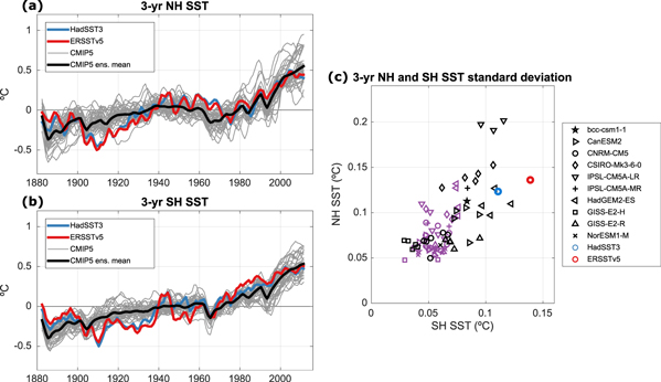
Figure 8. Consistency between simulated and observed changes in hemispheric-wide SST. (a) Northern hemisphere (NH) and (b) Southern Hemisphere (SH) running 3 year annual mean (December–November) time series of SST anomalies from 1881 to 2012 for HadSST3 (Kennedy et al 2011a, 2011b) and ERSSTv5 (Huang et al 2017) observations and CMIP5 historical simulations. CMIP5 results are based on 36 realizations from 10 models and masked to HadSST3's early-20th century coverage (Friedman et al in review). Thin lines show individual realizations; the solid black line shows the multi-model ensemble mean. (c) Comparison of NH and SH 3-year SST standard deviations. The CMIP5 historical ensemble mean is subtracted from the observations and the historical realizations, shown in black. Purple markers show standard deviations of 132-year pre-industrial control segments from the 10 CMIP5 models. Red and blue rings indicate observational estimates.
Download figure:
Standard image High-resolution imageTo what extent this discrepancy is due to model error, residual forcing or remaining observational error in SSTs (Chan and Huybers 2019, Haustein et al 2019) is presently unclear (Friedman et al in revision). The difference between variability with multimodel mean removed compared to that from control simulations (figure 8(c)) suggests that residual forcing may have contributed to the variability in observations. However, there is a wide range of simulated variability amplitudes in the CMIP5 models, even on the global scale (Knutson et al 2013, Schurer et al 2013, Sutton et al 2015). We conclude that, evaluating which, if any, of the climate models simulate reliable variability on decadal timescales is difficult—both due to limited sampling in observations, and the difficulty to separate forced response from internally generated variability. This should be a high priority for research.
5. Example of long-term changes on local weather variability
Lastly, the large-scale changes over the instrumental period also had a demonstrable impact on local weather variability that would have affected society and ecosystems. Individual extreme events occurred in the past, and their analysis and attribution is an area that is of developing interest. For example, the European 'year without a summer' had a clear impact from the Mount Tambora eruption which greatly enhanced the probability of such a cold summer as occurred in 1816 (Schurer et al 2019). The Dust Bowl heat waves in the central United States in the 1930s set records to date (Donat et al 2016, Cowan et al 2017), and have likely been strongly influenced by changes in land cover (Cowan et al in prep.) consistent with sensitivity of land climate to vegetation and land degradation (Arneth et al 2019). The 1947 European heat wave (Harrington et al 2019) record was only superseded in 2003. Figure 9 illustrates that long-term changes are detectable even in day-to day variability: many record-cold winter temperatures that occurred early on in Uppsala, Sweden, would be considered extremely rare at present, while some recent warm temperatures were rare in the past, and the distributions of daily temperature diverge significantly (based on a Mann–Whitney U test) between the three analysis periods of the early 19th century, early 20th century and recent period. Almost for every day of the year for Central England, and for most of those for the Uppsala record, the day-to-day variability is significantly different today from what it was 200 years ago, and for about half the year the change between the early 20th century warm period and the present is significant. The figure also illustrates the challenges of old records: the higher 90th percentile for peak summer values early on in the Uppsala record may possibly have been due to changes in instrument exposure (Moberg et al 2003). Studying old record-setting events will help to better understand the magnitudes and feedbacks of climate variability and extreme events.

Figure 9. Long-term change in daily temperature variability. Daily temperatures (°C) plotted against [day/year] from (a) the Central England time series (Parker et al 1992) and (b) Uppsala, Sweden (see text; Moberg et al 2002). Rings are individual years, and lines represent the 10th and 90th percentiles based on smoothed (11-day averaged) daily climatology. Bars on top illustrate where three periods considered show significantly different daily temperature distributions (based on a Mann–Whitney U test): the early 19th century (1790–1820, blue; with daily data cyan; blue bar on top where different from recent, red where different from early 20th century), the early 20th century (1920–1950, red, daily data yellow; grey bar on top where significantly different from recent) and the recent period (1980–2010, black, daily data grey). Note significant changes across much of the seasonal cycle between all periods with strong change in winter extremes.
Download figure:
Standard image High-resolution image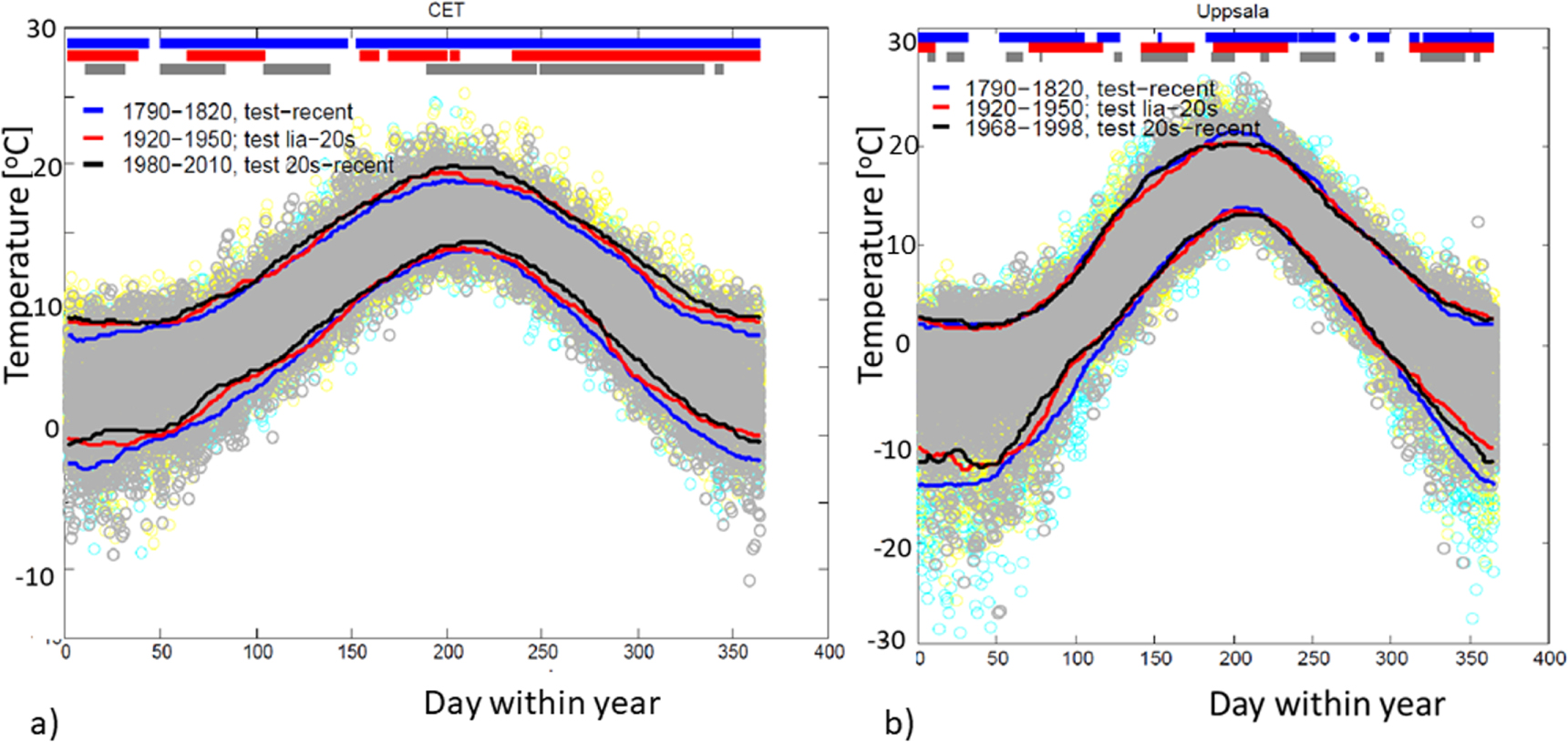
6. Synthesis and open questions
We have summarized that both external forcings and decadal climate variability have played a key role throughout the instrumental era. Greenhouse gas increase emerges as important throughout, supported by the analysis of proxy based data, and had already caused a detectable warming by 1900. The analyses also emphasize that the anthropogenic warming trend can be modified strongly both by natural forcing, and by climate variability, either on decadal timescales or due to decadal preferences of interannual modes, as here illustrated for the NAO. The period prior to 1950 contains strong variability (some of which may be realistic rather than data artefacts), cases of very strong natural forcing, and substantial changes in daily climate variability.
Hence the observed record in its full length contains vital information. It also has great potential to provide a constraint on future warming, and this has been used, for example, as one of several inputs to derive uncertainty ranges for IPCC projections (Knutti et al 2008, Collins et al 2014; using the Stott and Kettleborough 2002, approach) and recently in Goodwin (2018) and Goodwin et al (2018), generating observationally constrained projections. However, the power of attributed greenhouse warming for providing constraints is limited due to the still highly uncertain influence from other anthropogenic forcings, most notably, aerosols. Aerosols increased along with the burning of fossil fuels, yet burdens in Europe and North America noticeably decreased since the late 20th century, while continuing to increase in South and East Asia (Hoesly et al 2018), with a global peak of sulphate aerosol emissions around 1980. Aerosols have likely influenced global temperatures with a heterogeneous pattern and larger changes near and downwind of their emission regions, diurnal temperature range, and possibly even multi-decadal variability of the Atlantic as well as the large-scale atmospheric circulation. A particularly important impact of aerosols has been on monsoons and tropical rainfall. Land use change may be important as well, for example, on summertime extreme events (e.g. de Noblet-Ducoudré et al 2012). Land use change is not necessarily realistically simulated in climate models (Pitman et al 2009). For a more reliable attribution and prediction of regional scales, the inclusion of land use effects is vital and progress may arise from a CMIP6 modelling exercise Land Use Model Intercomparison Project (LUMIP; Lawrence et al 2016).
Decadal modulation of greenhouse warming trends over the industrial period often involved natural forcings, particularly volcanism, which is able to drive periods of decadal and multidecadal warming and cooling trends. The contribution by volcanism to temperature trends is particularly pronounced in the early 19th century. The large response illustrates that strong volcanic forcing would have a considerable impact on future warming trajectories.
Instrumental records of precipitation change are only reasonably widespread since the 1920s (Zhang et al 2007), and the signal-to-noise ratio for precipitation data is low and local variability high. Yet, if aggregated skilfully, long records have the potential to allow useful evaluation of the model simulated precipitation response, and the improvement of data coverage and a better understanding of long-term homogeneity will be helpful.
Analysis of the influence of circulation on observed trends shows a role of, possibly random, decadal modulation of modes of variability such as the NAO. While optimal detection should be able to reduce the influence of internal variability, rotating away from noisy spatial dimensions (Hasselmann 1979) or prewhitening noisy data (Allen and Tett 1999); in practice the limit on the space-time degrees of freedom that can be used in these methods is so severe that this advantage cannot fully be taken advantage of, even for recent methods (e.g. Ribes and Terray 2013, Ribes et al 2017). Hence reliance on statistics alone to filter out the influence of modes of variability on forced signals is not sufficient, and explicit analysis of changes in modes of variability is useful. Also, the question remains as to what extent variations in modes of climate variability are induced by external forcing. This is uncertain not only in response to anthropogenic factors, but also in response to natural forcings. For example, volcanic eruptions are expected to cause a tendency for a positive NAO response as well as a possible El Niño response (Robock 2000, Khodri et al 2017, Swingedouw et al 2017), although the response can be quite noisy (Hegerl et al 2011, Polvani et al 2019). Similarly, the relationship between solar forcing and the NAO is not yet fully understood (Gray et al 2010). Addressing the connection between external forcing and the response in modes of variability as well as circulation features is a priority, and one which may not be well addressed by the present generation of climate models (Shepherd 2014). In the near-term, climate variability will have a strong imprint on the emerging climate change signal in many regions (Deser et al 2017), and hence evaluation of this long term variability is crucial. A careful evaluation of data quality as well as climate model processes may, for example, help to determine whether the strong early variability in the Southern Hemisphere in observations is realistic.
In summary, the record of observed and reconstructed climate over the industrial period contains important information to challenge and evaluate climate model simulations. Even though data from the longer past are more challenging to work with due to their poorer spatial resolution as well as homogeneity issues, the gain is well worth the effort.
7. Methods
7.1. Literature search
This review focuses largely on identifying answers to key research questions about the instrumental era from existing literature; involving a broad set of coauthors to cover it well, and it includes new results that are being published. Additionally, web of science searches have been conducted to ensure broad coverage, using the keywords.
'Detection and Attribution, global temperature'; using outcomes from 2012 onwards as IPCC WGI will have captured results prior to that. A further search term was '19th century global temperature change'.
7.2. Construction of figure 1: Merging of PMIP and CMIP multimodel simulations
Global mean temperature in all simulations is calculated as a blend of surface air temperature over land and sea-surface temperature over ocean with full coverage. To account for a potential difference in the sensitivity of forcings in the multi-model-means (MMMs) drawing on a different ensemble of climate models, the last millennium MMM is regressed onto the CMIP5 MMM during the period of overlap using a total least squares regression (scaling factor 1.20). The last millennium MMM is then scaled by the regression factor and is re-normalised so that it has the same mean over the shared period 1861–1999 as the CMIP5 MMM, where the CMIP5 MMM is plotted as anomalies since 1961–1990.
Acknowledgments
This work has benefitted from fruitful discussions with Tom Delworth, Hugues Goosse, Philip Brohan, Debbie Polson, Massimo Bollasina, and Simon Tett. AS, ARF, SU, TC, CI and GH were supported by the ERC funded project TITAN (EC-320691). AS and GH were further supported by NERC under the Belmont forum, grant PacMedy (NE/P006752/1), and GH was by the Wolfson Foundation and the Royal Society as a Royal Society Wolfson Research Merit Award (WM130060) holder and by the NERC-funded SMURPHS project. SB was supported by the ERC funded project PALAEO-RA (787574).
We acknowledge the World Climate Research Programme's Working Group on Coupled Modelling, which is responsible for CMIP, the climate modelling groups for producing and making available their model output, the US Department of Energy's Program for Climate Model Diagnosis and Intercomparison, and the Global Organization for Earth System Science Portals for Earth System Science Portals.
Data availability statement
Data sharing is not applicable to this article as no new data were created or analysed in this study. Graphs shown in the study are either based on studies published elsewhere, or derived from data publically available including from JASMIN (for CMIP5 results) and observational data providers. Derivation of graphs that are not directly from other papers is described in detail in the paper; but time series shown can be provided from the first author on reasonable request.