

Abstract
Production of biomass for bioenergy can alter biogeochemical and biogeophysical mechanisms, thus affecting local and global climate. Recent scientific developments have mainly embraced impacts from land use changes resulting from area-expanded biomass production, with several extensive insights available. Comparably less attention, however, has been given to the assessment of direct land surface–atmosphere climate impacts of bioenergy systems under rotation such as in plantations and forested ecosystems, whereby land use disturbances are only temporary. Here, following IPCC climate metrics, we assess bioenergy systems in light of two important dynamic land use climate factors, namely, the perturbation in atmospheric carbon dioxide (CO2) concentration caused by the timing of biogenic CO2 fluxes, and temporary perturbations to surface reflectivity (albedo). Existing radiative forcing-based metrics can be adapted to include such dynamic mechanisms, but high spatial and temporal modeling resolution is required. Results show the importance of specifically addressing the climate forcings from biogenic CO2 fluxes and changes in albedo, especially when biomass is sourced from forested areas affected by seasonal snow cover. The climate performance of bioenergy systems is highly dependent on biomass species, local climate variables, time horizons, and the climate metric considered. Bioenergy climate impact studies and accounting mechanisms should rapidly adapt to cover both biogeochemical and biogeophysical impacts, so that policy makers can rely on scientifically robust analyses and promote the most effective global climate mitigation options.
Export citation and abstract BibTeX RIS

Content from this work may be used under the terms of the Creative Commons Attribution-NonCommercial-ShareAlike 3.0 licence. Any further distribution of this work must maintain attribution to the author(s) and the title of the work, journal citation and DOI.
1. Introduction
1.1. Background
Recent life-cycle assessment (LCA) studies of bioenergy systems have mainly focused on the contributions from direct and indirect land use change (LUC) effects, quantifying the unit-based impacts of indirect GHG emissions resulting from area-expanded biomass production for bioenergy and related market-mediated effects [1–5]. Relatively less attention is given to the direct climate performance of bioenergy systems from rotation forestry or plantations, where land use-induced climate forcings are temporary.
Concerning biogeochemical effects, i.e. those related to the carbon cycle, the majority of environmental impact studies and bioenergy policies treat direct CO2 emissions from regenerative biomass under the so-called 'carbon neutrality' convention: CO2 emissions are offset by CO2 sequestration in growing biomass, making bioenergy climate neutral. Both in the scientific [6–9] and policy community [10–12] there is an increasing qualitative perception about the inadequacy of assigning a Global Warming Potential (GWP) of zero to biogenic CO2 emissions, neglecting the climate forcing effects from temporary changes in atmospheric CO2 concentration. Forest carbon dynamic studies [13–15] long acknowledged these shortcomings, but limited solutions exist for emission metrics, unless simply equating the impact from biogenic CO2 to that of fossil CO2 using a GWP of one.
The importance and complexity of the topic is measured by the ongoing debate in the US, where the treatment of biogenic CO2 emissions from bioenergy in regulatory acts is currently under review [12]. Letters to the US House of Representatives (among others) by two prominent groups of US academics perfectly summarize the two major conflicting opinions: one group highlights 'the importance of accurately accounting for CO2 emissions from bioenergy in any law or regulation' [16], while the other expresses concerns in 'equating biogenic C emissions with fossil fuel emissions' [17]. In 2011, the US Environmental Protection Agency (EPA) opted for a three-year deferral of the so-called final greenhouse gas (GHG) 'tailoring rule' to biogenic CO2 emissions from bioenergy, motivating this choice with the need to effectuate a survey of the existing scientific literature [12].
Further adding to the discussion are concerns surrounding changes in biogeophysical climate regulatory factors associated with bioenergy production, such as changes in surface reflectivity (albedo), evaporation/transpiration, and surface roughness, which can play an important role in regulating surface energy fluxes and the hydrologic cycle [18, 19]. A change in land use to produce crops for bioenergy can alter these factors in complex ways that can either enhance or offset C cycle climate impacts, depending on local climate variables and vegetation dynamics. Even if recent studies demonstrate their importance for local climate when bioenergy is produced from crops and plantations expanded on former agricultural land or grassland [20–26], they are often overlooked in most bioenergy LCA, existing climate policies, and methodological standards [10]. This may be attributed in part to the inherent complexity of combining local with global and direct with indirect climatic effects into meaningful metrics, and in part to the fact that many biogeophysical land use forcings cannot be reliably or efficiently measured [19, 27, 28]. Changes in evaporation/transpiration and other factors do have an impact on local climate, but cannot be adequately quantified in terms of global radiative forcing [29–31], which is a measure of the global warming or cooling potential of any anthropogenic or natural forcing [30, 32]. Comprehensive assessments including the totality and complexity of global and local climate implications would be ideally needed for the most informed decision making, yet it is possible to arrive at insightful conclusions by focusing efforts on direct global climate implications through changes in the Earth's radiative balance, which is the main driver for the climate system [21, 29, 33–35]. On the global scale, the albedo effect is found to be the dominant direct biogeophysical climate forcing, particularly in areas affected by seasonal snow cover [31, 35–37], and can be compared to the effects of GHGs using radiative forcing (RF) as a metric basis [19, 29, 35, 37–40].
1.2. Aim of the study
The aim of this paper is to assess the contributions to direct global warming of various bioenergy case studies from temporary climate forcings as changes in atmospheric CO2 concentration and surface albedo, in addition to direct greenhouse gas (GHG) emissions throughout the value chain. The analysis focuses on CO2 from bioenergy sourced from a stand where biomass is kept under continuous rotation (no land use change), and an LCA perspective is undertaken. Using empirical data and relatively simple climate models, we advance former approaches and report insightful findings from case studies spanning a diversity of geographical regions and biomass species: (a) USA—forest wood from managed, high-productive sites in the Pacific Northwest (PNW) and in northern Wisconsin (WI); (b) Canada (CA)—managed forest wood; (c) Norway (NO)—managed forest wood, both with 'NO (fr)' and without 'NO' forest residue removal; (d) fast growing species like eucalyptus in Brazil and willow in the EU and US. Results are presented in both absolute and more commonly accepted emission metrics like GWP, using instantaneous and time-integrated effective radiative forcing as a basis [32, 41–43].
2. Methodology
In the next sections, the methodology used to quantify the contributions to global warming of biogenic CO2 fluxes and changes in albedo is described. Impacts under study are from vegetation dynamics on lands currently under biomass management for bioenergy, such as existing forests and plantations, under a single stand perspective. Specific details and information about geographic locations, climatic conditions, biomass species, uncertainty analysis of key parameters, and life-cycle GHG emissions of the selected case studies are available in the supplementary data (available at stacks.iop.org/ERL/7/045902/mmedia). In our work, we use the term 'biogenic CO2' to refer to CO2 fluxes circulating between the vegetation and the atmosphere, i.e. CO2 from oxidation of carbon in bio-materials harvested for energy (both at the conversion plant and through the various life-cycle stages) and dead organic matter decomposition, and CO2 sequestered by growing biomass.
2.1. Biogenic CO2 fluxes
Changes in atmospheric CO2 concentration following emissions can be modeled using an impulse response function (IRF) [44–47], which is a simple useful outcome of carbon-cycle climate models of varying complexity. This function describes the fraction of CO2 remaining in the atmosphere after a single pulse emission, according to the interactions with the oceans and the terrestrial biosphere. A modified IRF needs to be elaborated for modeling the atmospheric decay of biogenic CO2 emissions sourced from regenerative biomass, in order to take into account the dynamics of the biogenic CO2 fluxes involved and their interactions with the global carbon cycle [8, 48–50]. Once in the atmosphere, CO2 molecules of biogenic origin are identical to fossil-derived CO2 molecules, but the time profile of the decay is different. If sourced from biomass land kept under management, biogenic CO2 has the additional flux inherent to biomass-based energy systems, i.e. the sequestration of CO2 by growing vegetation, acting to further reduce atmospheric CO2 concentration. Clearly, this difference fails when biomass is sourced from a deforested area. Timing of fluxes is therefore crucial for the climate impact of bioenergy: emissions generally occur at a single point in time, while the sequestration flux is a function of the biomass rotation period, varying from one year for annual crops to several decades for forest biomass. Such a time gap between biogenic CO2 fluxes is responsible for a certain climate impact of bioenergy, even if the system is carbon neutral over time.
Emissions from harvested biomass for bioenergy are modeled as a single pulse using a delta function, following common practice in the bioenergy literature [49, 51–53]. Rather than the simple forest growth rate used in former studies [8, 48–50], site-specific chronosequences of net ecosystem productivity (NEP) are used here for modeling CO2 dynamics from the site after harvest. NEP profiles have the key advantage of being measured on field and inclusive of all CO2 exchanges between the atmosphere and the forest, comprehensive of all the different forest carbon pools. In terrestrial ecosystem studies, NEP is defined as the rate of change in ecosystem C storage over time [54–56], and is the difference between CO2 sequestered through net primary production (NPP) and released through heterotrophic respiration (i.e. soil respiration and decomposition of dead organic materials, such as forest residues, left on site after harvest). Whenever possible, we adopt empirical NEP values measured on field with flux towers through the eddy covariance technique, which provides a direct method to investigate the ecosystem–atmosphere C exchange of whole ecosystems [57–59]. NEP changes as a function of time are then elaborated through chronosequences, which is a collection of data from forest stands of different age but otherwise homogeneous for plant material and environmental conditions. Where a chronosequence was not available, NEP was indirectly modeled using carbon dynamic models that simulated time-dependent responses of ecosystems to harvest disturbances and a set of site-specific stand parameters and meteorological data. In these cases (Norwegian forest, eucalyptus, and willow), the decay rates of forest residues left on the forest after harvest are firstly modeled and then subtracted from NPP to get the NEP curve. Additional specific information is available in the supplementary data (available at stacks.iop.org/ERL/7/045902/mmedia). NEP dynamics are from secondary succession and carbon neutral along the rotation period. The NEP status of a stand varies over time depending on which process dominates, photosynthetic production or respiration: when NEP is positive, the ecosystem is a CO2 sink, when negative it is a CO2 source. In the investigated stands, we observe an initial period dominated by C losses (negative NEP) where CO2 emissions from dead organic material decomposition exceed CO2 sequestration, with the ecosystem being a carbon source (in the case of forests, this period may last for a couple of decades). As dead organic material decomposes away and sequestration of carbon from growing biomass increases, NEP switches from negative to positive and the ecosystem becomes a carbon sink until the new harvest event. Because the stand is kept under continuous management, the overall system is modeled as being carbon neutral over the rotation period: what is emitted through combustion and oxidation is sequestered again by growing trees during the rotation period.
These biogenic CO2 fluxes cause a change in atmospheric CO2 concentration, obtained through the following convolution (valid when emissions for bioenergy are modeled with a delta function at year zero) [8]:

where t' is the integration variable from the time since harvest, t is the time dimension, NEP(t') is the function representing the CO2 flux rate from the site after harvest (normalized to the unit pulse), and y(t) is the IRF from the carbon-cycle climate model (parameterized with the values reported in the 4th IPCC report [32]). The function f(t) describes the time-dependent changes in atmospheric CO2 concentration from biogenic CO2 fluxes, i.e. the site-specific IRF describing the atmospheric decay of biogenic CO2. This is the basis for the estimation of the resulting impact on global warming through the concept of RF, which is the perturbation of the earth's energy balance at the top of the atmosphere (TOA) by a climate change mechanism. The time evolution of RF from a unit pulse emission at time zero is proportional to the atmospheric decay of the gas, here calculated through radiative efficiencies assumed to be constant over time [32].
2.2. Changes in surface albedo
Changes in surface albedo occur after biomass harvest (especially forests), when the solar reflective property of the surface is perturbed, and are of significance in regions affected by seasonal snow cover [36, 37, 60]. This temporary perturbation causes a cooling contribution thanks to the higher reflective property of snow than forest canopy and is a function of the biomass rotation period when albedo reverts back to the pre-harvest value after a certain time. A global radiative forcing over time from a temporary surface albedo change can be described by the following equation (updated from [48]):

where  is the mean incoming solar radiation at the top of the atmosphere (TOA) in month m for a given site (in W m−2),
  is a two-way atmospheric transmittance parameter accounting for the monthly mean reflection and absorption of solar radiation (downward and upward) throughout the atmosphere for the same site and month,
  is the difference in monthly mean surface albedo between standing biomass and the clear-cut site, Aaff is the local area affected, M is the total number of months, yα(t) is a function describing the interannual time evolution of the annually averaged local instantaneous forcing, and AEarth is the area of the Earth's surface.
MODIS black-sky shortwave broadband (near infrared and visible) albedo data (Collection 5, MCD43A) were obtained from the MODIS subset data server for all sites with a spatial resolution of approximately 0.25 km2 [61]. Individual image data sets are eight-day composites of atmospherically corrected surface reflectance, derived by using cloud-free images only [62]. For any eight-day composite with no retrieval of acceptable quality, albedo is estimated based on linear interpolation between succeeding and preceding composites. Whenever possible, albedo data for multiple years are compiled and averaged together to reduce uncertainty associated with annual variability in phenology and local climate.
The two-way atmospheric transmittance  parameter is estimated as the product between
  , the average fraction of downwelling solar radiation at TOA reaching the Earth's surface in month m, and Ta, the fraction of reflected radiation at the surface arriving back at TOA. For
  , we rely on 22 year mean monthly insolation clearness index data provided by NASA's Solar Surface Energy project for each of our specific site locations [63]. For Ta we use a global annual average of 0.854 [64], whose suitability is tested by comparison with a more parameterized plane-parallel radiative transfer model (the Fu–Liou model [65]) using the Canadian case as an example (see figure S5 in the supplementary data available at stacks.iop.org/ERL/7/045902/mmedia).
The incoming solar radiation at the TOA on any given Julian day of the year from 1 to 365 can be calculated by knowing latitude L in degrees, the declination angle δ in degrees, and the sunset hour angle ω in degrees [66, 67], following equations reported in [48].
The variable yα(t) of equation (2) describes the time evolution of the local albedo change forcing at any future time step relative to the initial change at the time of disturbance (i.e. a clear-cut harvest). Following empirical observations showing that albedo decreases exponentially over the biomass rotation period [68, 69], with more rapid decreases occurring in the first 30%–50% of the rotation period, we use a simple first-order decay model for yα(t), with the mean lifetime at 1/5th of the rotation period. Albedo change forcings are assumed negligible for fast growing biomass species, owing to the short rotation time scales involved, and for biomass sourced from areas not affected by seasonal snowfall.
2.3. Direct GHG emissions through the life-cycle
Direct life-cycle GHG emissions throughout the bioenergy value chains are also considered in this study. Common first generation biofuels and fossil fuels are assessed in order to benchmark our results. Both in the US and EU these energy products are well established in the market and their performances in terms of GHG emissions are extensively documented in primary research studies and standardized in regulations and guidelines [70, 71]. We therefore rely on the standard values therein reported. When more than one option is available, the most promising and optimistic results are considered. Contributions from indirect/market-mediated effects are not included (and set to zero if present in the data gathered). In all cases, the analysis covers the three 'Kyoto gases' CO2, CH4 and N2O and the various processing steps, whose impact is modeled using the IRF and radiative efficiencies reported by the IPCC [32]. Life-cycle stages considered are agricultural production or harvest (including fertilizers, irrigation, and mechanical operations), transport, conversion, and combustion. For transportation biofuels, fuel distribution and filling station operations are excluded in order to standardize the results. Specific references and key parameters are available in the supplementary data (available at stacks.iop.org/ERL/7/045902/mmedia).
2.4. Climate metrics
Two main types of climate metrics can be identified, in relation to the treatment of time [43]: absolute metrics, which compare the climate impact caused by different emissions over time (e.g. change in atmospheric CO2 concentration, instantaneous and integrated radiative forcing), and normalized metrics, which quantify the climate impact relative to a reference gas (e.g. GWP). In the LCA community, the latter are the most common, even if additional insights can sometimes be provided by the former. In this paper, we report results according to both types of metrics.
Directly measuring climate effects from various forcings in terms of global RF implicitly assumes that the same forcings from different climate change mechanisms have the same climate response in terms of a global surface temperature change [42]. When climate forcings like changes in albedo are assessed together with GHGs, the non-negligible differing climate efficacies should be taken into account. In the selected case studies, the major albedo changes occur during the winter months (see figures S8–S12 available at stacks.iop.org/ERL/7/045902/mmedia in the supplementary data, first graph: clear-cut versus forested land), when land is covered by snow. Several experiments and simulations clearly show that the climate response to 1 W m−2 of forcing from CO2 significantly differs from that of the same forcing due to a change in snow albedo, which is from 1.5 to 5 times more effective than CO2 in affecting global surface temperature, depending on specific conditions and modeling assumptions [60, 72–75]. In order to consider these differences, we use the climate efficacies E (ECO2 = 1,ECH4 = 1.33,EN2O = 1.17 and Ealbedo = 1.94) obtained from numerical climate simulations elaborated after investigation of the many climate forcings affecting global climate [60]. The reference climate sensitivity of CO2 is that resulting from an increase of 1.25 of the preindustrial CO2 atmospheric concentration (290 ppmv). This choice is due to the need for consistency with the IRF used to describe the decay of CO2 in the atmosphere, which is defined for a constant background concentration of 378 ppmv. This enables a consistent comparison of the various forcing agents in terms of their 'effective radiative forcing' [60, 73].
The normalized metric GWP, inclusive of climate efficacies, can then be computed for the different GHGs, including biogenic CO2, and the most common time horizons (TH), 20, 100, and 500 years:
A characterization factor for a surface albedo change when biomass is harvested for bioenergy is the ratio of the time-integrated radiative forcing from the albedo change per m2 affected area (i.e. clear-cut area) relative to that of a 1 kg pulse anthropogenic CO2 emission over the same time horizon (TH) normalized to the carbon yield γ (in kg-bioCO2 m−2 of affected area) on the same land area:

3. Results and discussion
Contributions to global warming of biogenic CO2 fluxes, changes in surface albedo, and life-cycle GHG emissions, are shown in the next sections both in terms of absolute and normalized metrics (GWP). After that, results from an improper characterization of biogenic CO2 emissions are discussed. Additional results are available in the supplementary data (available at stacks.iop.org/ERL/7/045902/mmedia).
3.1. Absolute metrics
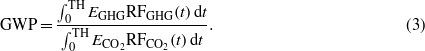
Supplementary figure S1 (available at stacks.iop.org/ERL/7/045902/mmedia) shows the IRFs (or changes in atmospheric CO2 concentration) of biogenic CO2 emissions for the different biomass feedstocks, in comparison with a CO2 pulse emission from fossils or deforested biomass (here ideally intended as biomass released to the atmosphere at one point in time and sourced from an area that is not re-vegetated). Figure 1 shows the resulting instantaneous effective radiative forcing associated with a pulse emission of CO2 from biogenic CO2 fluxes and changes in surface albedo for the different bioenergy options. These effects are temporary, and their instantaneous impacts approach zero in the long term. Time-integrated results are shown in supplementary figure S2 (available at stacks.iop.org/ERL/7/045902/mmedia).
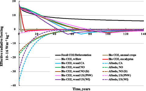
Figure 1. Effective radiative forcing (instantaneous) from biogenic CO2 fluxes (Bio CO2) and changes in albedo associated with one kg of emission for the different biomass feedstocks analyzed in this study. The effective forcing of a CO2 pulse emission from fossils or deforested biomass is shown for comparison. Abbreviations: PNW =Pacific Northwest (US); WI =Wisconsin (US); CA =Canada; NO =Norway; fr = with harvest of 75% of above ground forest residues.
Download figure:
Standard imageThe atmospheric decay of biogenic CO2 from fast growing species like willow and eucalyptus is faster than that from slow growing biomass. When biogenic CO2 emissions come from combustion of forest biomass, their atmospheric decay is slower than that of fossil CO2 for the first decades, due to the additional emissions from the site after harvest (where NEP is negative). Biogenic CO2 decays show a clear inflection point at the end of the rotation period, when biomass is harvested and NEP abruptly stops. The presence of negative values in the curves from biogenic CO2 fluxes is due to the interactions with the upper layers of the oceans, which slowly outgas the CO2 quickly absorbed soon after the pulse emission. This causes a postponement in the achievement of the neutrality in terms of changes in atmospheric CO2 concentrations (in mass terms the neutrality is reached at the end of the rotation period). Other papers have discussed this physical effect in more detail [8, 49, 51, 76].
The importance of the cooling contributions from albedo in areas affected by significant snow cover appear evident, especially for the Canadian, Wisconsin, and Norwegian case, while a smaller effect is observed in US PNW. Beyond local climate variables and vegetation dynamics affecting atmospheric transmittance of solar radiation, the magnitude of the albedo contribution can vary depending on the biomass yield per unit area affected, with the strength per kg of emission inversely proportional to the effect of increased yields. For example, while the harvest disturbance induces a similar local annual forcing for PNW and WI (−5.4 and −5.3 W m−2, respectively), the normalized albedo effect per unit of mass is much greater for the Wisconsin case where yields are approximately one tenth that of the PNW case. The effects of collecting forest residues are multifold and contrasting. On one side, the contribution to global warming from biogenic CO2 fluxes decreases (faster decay of biogenic CO2 in 'NO (fr)' than 'NO' case) thanks to a lower amount of dead organic material left on site to decompose; on the other side, the cooling from albedo is also reduced. This is the result of two contrasting effects. A larger change in albedo due to a smoother forest floor (less snow is required for a homogeneous solar radiation reflectivity) is more than offset by the higher biomass yield of the site, so reducing the area harvested per unit. The uncertainty analysis available in the supplementary data (available at stacks.iop.org/ERL/7/045902/mmedia) discusses the sensitivity of the magnitude of the albedo effect to the altitude of the site and other key parameters.
As discussed hereafter, the climate impact of bioenergy increases when the entire value chain is assessed due to contributions from fossil fuel emissions from life-cycle operations, upstream emissions through conversion processing and efficiency penalties, and lower energy densities of biomass compared with fossil fuels. Figure 2 shows the instantaneous radiative forcing profiles per MJ combusted of the selected case studies producing both heat from stationary applications and transportation biofuels (bioethanol and Fisher–Tropsch diesel). Figure 2(a) shows the dynamics of the effective forcing for bioenergy systems in comparison with fossil fuel-based systems (coal, oil, and natural gas) producing heat from stationary applications. In figure 2(b), transportation biofuels are compared to conventional fossil fuels such as diesel and gasoline. Supplementary figure S3 (available at stacks.iop.org/ERL/7/045902/mmedia) shows the single contributions of the different climate forcing agents to changes in the effective forcing (both instantaneous and integrated), exemplified with the WI case. The dynamics of the curves in figure 2 show the complexity of the systems and the large time dependency of the results. When a strong cooling contribution from albedo is present, the warming from biogenic CO2 fluxes can be more than offset in the short run, and bioenergy systems start with a net negative impact, i.e. a cooling effect. When the albedo effect is small, warming from biogenic CO2 fluxes clearly dominates, and bioenergy systems show a higher net impact than fossil systems for a period of time that ranges from a few years, for fast growing biomass species, to several decades, for slow growing biomass like forest wood. From the medium term (60–80 years) and beyond, the instantaneous climate impact of bioenergy systems gradually decreases and becomes smaller than that of fossil reference systems, even for transportation biofuels produced from forest wood that do not have the benefit of cooling effects from albedo.
Figure 2. Net effective radiative forcing (instantaneous) for the different bioenergy options for stationary (a) and vehicle (b) applications and fossil reference systems. Abbreviations: PNW= Pacific Northwest (US); WI= Wisconsin (US); CA= Canada; NO= Norway; fr= with harvest of 75% of above ground forest residues; FTD= Fisher–Tropsch diesel.
Download figure:
Standard image3.2. Normalized metrics
Table 1 shows GWP equivalency factors for the three most common time horizons of 20, 100, and 500 years, computed with time-integrated effective radiative forcings and using CO2 as reference. Biogenic CO2 emissions from biomass combustion (and from process losses) are multiplied by the respective GWP to get the resulting contribution to global warming. This also applies to the case where 75% of above ground forest residues are harvested with the stem (there is no distinction between residues and stems at the conversion plant). Thanks to these equivalency factors, LCA practitioners can treat biogenic CO2 as the other common GHGs, for which emissions are reported as inventory items and sequestration fluxes are included in the IRF that is the basis of the respective equivalency factor. For instance, in the emission inventory we report CO2 emissions from fossil fuels and not the amount of CO2 sequestered by the oceans. Similarly, only biogenic CO2 emissions from combustion or oxidation through the life cycle are to be noted in the emission inventory, while the sequestration fluxes are incorporated in the site-specific GWP.
Table 1. GWPs for the selected biomass case studies and time horizons. GWP values for CH4 and N2O differ from that reported in the 4th IPCC Assessment report [32] because here the effective radiative forcing is used as basis.
| GWP | |||
|---|---|---|---|
| 20 | 100 | 500 | |
| CO2 | 1.00 | 1.00 | 1.00 |
| CH4 | 96.3 | 34.5 | 10.6 |
| N2O | 336 | 348 | 179 |
| NO: Bio CO2 | 1.25 | 0.62 | 0.11 |
| NO: Albedo | −0.94 | −0.42 | −0.13 |
| NO: Net | 0.32 | 0.20 | −0.02 |
| NO (fr): Bio CO2 | 1.07 | 0.51 | 0.09 |
| NO (fr): Albedo | −0.85 | −0.38 | −0.12 |
| NO (fr): Net | 0.22 | 0.12 | −0.03 |
| US PNW: Bio CO2 | 1.04 | 0.58 | 0.10 |
| US PNW: Albedo | −0.14 | −0.07 | −0.02 |
| US PNW: Net | 0.90 | 0.51 | 0.08 |
| US WI: Bio CO2 | 1.08 | 0.32 | 0.06 |
| US WI: Albedo | −1.10 | −0.38 | −0.12 |
| US WI: Net | −0.02 | −0.06 | −0.06 |
| CA: Bio CO2 | 1.13 | 0.42 | 0.08 |
| CA: Albedo | −1.60 | −0.61 | −0.19 |
| CA: Net | −0.47 | −0.18 | −0.11 |
| Eucalyptus: Bio CO2 | 0.17 | 0.03 | 0.01 |
| Willow: Bio CO2 | 0.09 | 0.02 | 0.00 |
| Annual crops: Bio CO2 | 0.02 | 0.00 | 0.00 |
Contrary to the GWPs for the other GHGs, characterization factors of biogenic CO2 need to be assessed on a case-by-case basis, because carbon-cycle and albedo change dynamics are greatly affected by local conditions and biomass species. For TH = 20 years, some values of GWP from biogenic CO2 are higher than the one due to additional emissions from oxidation of dead organic materials left on site after harvest. Values are higher for systems where biomass is sourced from slow growing forests and for shorter THs, while they are significantly lower for fast growing biomass species and TH = 500 years. Cooling contributions from albedo are significant when biomass is sourced from forested areas affected by seasonal snow cover.
Figures 3 and 4 show the impact of global warming in g CO2-eq MJ−1 of fuel combusted for the selected THs for stationary and vehicle applications, respectively. For vehicle applications, both commercial first generation biofuels from annual crops and fossil fuels are shown to benchmark our results. Existing policy frameworks and methodological standards are only based on life-cycle emissions, displayed with black bars in figures 3 and 4. Contributions from biogenic CO2 and albedo, which are usually overlooked, far outweigh GHG emission impacts throughout the life-cycle in the cases when biomass is sourced from slow growing species and for a short TH.
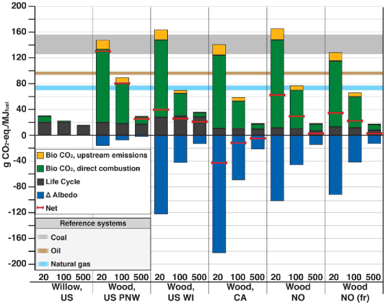
Figure 3. Direct contributions to global warming of the different bioenergy options for stationary applications. GWP factors, corrected with the climate efficacies of the various forcing agents, are used to characterize emissions, including biogenic CO2. Three time horizons (20, 100, and 500 years) are considered. Fossil fuels (coal, oil, and natural gas) per MJ of fuel combusted are shown to benchmark our results. Lower and higher limits of the bands for the fossil systems represent the impact for TH = 500 and TH = 20, respectively. Abbreviations: Bio CO2= biogenic CO2 emissions, i.e. emissions from oxidation of biomass harvested for bioenergy; upstream emissions= emissions from biomass losses through the value chain and biofuel processing; direct combustion= emissions from combustion of biofuels at plant; PNW= Pacific Northwest (US); WI= Wisconsin (US); CA= Canada; NO= Norway; fr= with harvest of 75% of above ground forest residues.
Download figure:
Standard image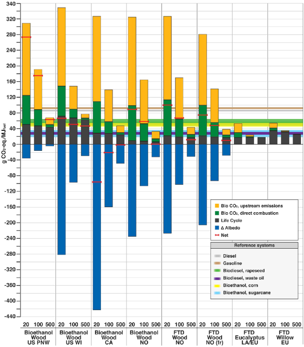
Figure 4. Direct contributions to global warming of the different bioenergy options for vehicle applications. GWP factors, corrected with the climate efficacies of the various forcing agents, are used to characterize emissions, including biogenic CO2. Commercial biofuels and fossil fuels per MJ of fuel combusted are shown to benchmark our results. Three time horizons (20, 100, and 500 years) are considered. Lower and higher limits of the bands for the reference systems represent the impact for TH = 500 and TH = 20, respectively. For annual crops, contributions from biogenic CO2 and albedo are minimal, and not displayed with independent bars here (see supplementary information available at stacks.iop.org/ERL/7/045902/mmedia). Abbreviations: Bio CO2= biogenic CO2 emissions, i.e. emissions from oxidation of biomass harvested for bioenergy; upstream emissions= emissions from biomass losses through the value chain and biofuel processing; direct combustion= emissions from combustion of biofuels in vehicles; PNW= Pacific Northwest (US); WI= Wisconsin (US); CA= Canada; NO= Norway; fr= with harvest of 75% of above ground forest residues; LA= Latin America; EU= European Union; FTD= Fisher–Tropsch diesel.
Download figure:
Standard imageContributions from biogenic CO2 are divided between those from direct combustion of the final form of the biofuel and those from upstream emissions due to biomass handling and conversion processes. Direct biogenic CO2 emissions can only be reduced by coupling stationary bioenergy with CO2 capture, while upstream biogenic CO2 emissions can decrease by improving conversion efficiencies at the various life-cycle stages.
When compared with fossil fuel-based heat production facilities (figure 3), most of the bioenergy cases outperform fossil fuel systems. For forest-based bioenergy this is due to the cooling contributions from albedo changes. An exception is the US PNW case, where contributions from albedo changes are small and values for TH = 20 are comparable to that of coal.
Figure 4 shows that transportation biofuels are burdened by larger carbon emissions from upstream processing than stationary applications, with the sum of the yellow and green bars being around twice that of the heat options. This is due to the lower energy efficiency of the modeled conversion technologies for vehicle applications, which range between 40%–55%. For fast growing biomass species like eucalyptus and willow, direct global warming effects are comparable to biofuels from annual crops. For slow growing biomass feedstocks like forest wood, cooling from albedo change in the Canadian case more than offsets the warming from biogenic CO2 fluxes and direct life-cycle emissions. The impact of biofuels is higher than fossil fuels when biomass is sourced from slow growing forests where cooling contributions from albedo change are small, such as in the US PNW case. For longer TH, contributions from the temporary climate effects gradually decrease.
3.3. GWP of biogenic CO2: 0, 1, or site-specific?
Supplementary figure S4 (available at stacks.iop.org/ERL/7/045902/mmedia) shows the differences obtained by approximating the GWP of biogenic CO2 emissions with either a 0 or 1 factor neglecting temporary forcings, rather than using the site-specific GWPs computed in this study (represented by the horizontal axis). This analysis shows that substantially misleading conclusions can be achieved if biogenic CO2 emissions are improperly characterized, irrespective of the type of biomass and albedo contributions, and using either an equivalency factor of zero, stemming from the carbon neutrality convention, or one derived from simply equating the climate impact of biogenic to fossil CO2. In such cases, the direct impact to global warming of bioenergy can be over- or underestimated up to one order of magnitude. Such improper accounting can evidently result in very ineffective and counterproductive mitigation efforts. As shown in this paper, bioenergy climate impact studies should not be based on simple accounting conventions, given that the situation is far more complex than a simple matter of 0 or 1 accounting.
4. Conclusions
This analysis elaborated on the inclusion in bioenergy LCA of the contributions to global warming from temporary effects, such as changes in atmospheric CO2 concentration and surface albedo, for a variety of bioenergy systems. The focus on direct global impacts and the use of the effective radiative forcing as a basis for climate metrics ensures the advantage of expressing results both with absolute and normalized metrics (i.e. in terms of g CO2-equivalents per MJ). The influence on final results of these direct effects can be large, especially for short TH and when biomass is sourced from slow growing biomass species and areas affected by seasonal snow cover. Given the importance of site-specific considerations concerning vegetation dynamics and climatic aspects, GWPs of biogenic CO2 emissions are case specific. As one example, albedo contributions for US WI and US PNW significantly differ, even if the sites approximately have the same latitude and altitude. The need for high site-specific modeling resolution can give rise to issues regarding applications of GWPs for biogenic CO2 on a routine and transparent basis. However, equivalency factors such as those computed here can be derived for the most promising bioenergy locations and biomass species, after an optimization of the methodology described in this paper and documented in the supplementary data (available at stacks.iop.org/ERL/7/045902/mmedia).
In this study, the direct climate performance of bioenergy systems with respect to fossil reference systems depends on the type of metric considered, whether instantaneous or time integrated. Bioenergy systems generally have a lower impact when instantaneous metrics are considered, rather than integrated metrics as GWP. In general, impacts for bioenergy are higher for short TH, and tend to considerably decrease over time. However, when cooling contributions from albedo are strong, bioenergy systems can have a net negative global warming contribution (i.e. a net global cooling effect), even at the beginning of the assessment period. Bioenergy stakeholders at different levels should consider the complexity of the results, and their variation with respect to biomass species, geographical locations, temporal boundaries, climate forcing agents, and climate metrics. The ultimate climate assessment of a bioenergy system can also be affected by issues not covered by this analysis, such as local biogeophysical impacts, dynamics at landscape level, and other possible indirect/market-mediated effects. LCA studies and climate accounting mechanisms such as the Kyoto protocol and its successor should therefore transparently acknowledge these issues and urgently adapt to routinely incorporate those climate forcings that are generally the most significant at a global level, such as timing of biogenic CO2 fluxes and albedo changes.
Acknowledgments
We thank the Norwegian Research Council for funding this work through the Cenbio and ClimPol Projects. Thanks to Geoffrey Guest (NTNU) for sharing data on simulations of decay rates and to Dr Richard Plevin and Professor Michael O'Hare (UC Berkeley) for their critical review and comments.