

Abstract
With the emerging nationwide availability of battery electric vehicles (BEVs) at prices attainable for many consumers, electric utilities, system operators and researchers have been investigating the impact of this new source of energy demand. The presence of BEVs on the electric grid might offer benefits equivalent to dedicated utility-scale energy storage systems by leveraging vehicles' grid-connected energy storage through vehicle-to-grid (V2G) enabled infrastructure. It is, however, unclear whether BEVs will be available to provide needed grid services when those services are in highest demand. In this work, a set of GPS vehicle travel data from the Puget Sound Regional Council (PSRC) is analyzed to assess temporal patterns in vehicle use. These results show that vehicle use does not vary significantly across months, but differs noticeably between weekdays and weekends, such that averaging the data together could lead to erroneous V2G modeling results. Combination of these trends with wind generation and electricity demand data from the Electric Reliability Council of Texas (ERCOT) indicates that BEV availability does not align well with electricity demand and wind generation during the summer months, limiting the quantity of ancillary services that could be provided with V2G. Vehicle availability aligns best between the hours of 9 pm and 8 am during cooler months of the year, when electricity demand is bimodal and brackets the hours of highest vehicle use.
Export citation and abstract BibTeX RIS
1. Introduction
The past decade has seen significant investment in renewable electricity generation across the United States [1]. While sustained growth could continue, wind and solar generation are highly variable resources, and are often not well matched to times of peak electricity demand [2]. The variability and temporal mismatch between electricity demand and renewable generation is currently moderated using ancillary services—backup generation provided by facilities operating at less efficient part-load levels (spinning reserve) and fast-response standby generators (non-spinning reserve), often aeroderivative gas turbines [3]. As the percentage of total capacity constituted by renewable generators increases, it is expected that reserve capacity must necessarily increase as well [4, 5]. Presently, low natural gas prices make backup generation from gas turbines a cost-effective option. Alternatively, energy storage could be used to provide low- or zero-emission backup power for renewables instead of gas turbines [6–8]. Further, gas turbine backup generation cannot offer the full range of benefits of energy storage, including improving the capacity factors of existing thermal generators and the utilization of existing transmission capacity, as well as peak shaving, peak shifting and firming of renewable generation [9]. Unfortunately, even accounting for the wide range of benefits that can be monetized, the capital costs of existing grid-scale storage technologies are prohibitive for most applications [10, 11].
In the past few years, several major automakers have begun series production of electric vehicles (EVs) and plug-in hybrid electric vehicles (PHEVs). Tax incentives, zero-emission vehicle mandates, decreasing battery costs and other factors portend battery electric vehicle (BEV) uptake in the coming years [12, 13]. From the standpoint of utilities and system operators, the presence of BEVs on the electric grid could offer an opportunity to use vehicle batteries as a form of distributed energy storage and capture benefits equivalent to dedicated utility-scale energy storage systems, while avoiding the prohibitive capital costs of traditional storage [14, 15]. It has been envisaged that vehicle owners could receive compensation for participation in a vehicle-to-grid (V2G) program, partially offsetting the cost of their vehicle's battery and any battery life effects that might be caused by such a program [14–16]. Ancillary services (AS) such as frequency regulation and spinning reserve services are often cited as the best revenue opportunity for vehicle owners because they can receive capacity payments and the power and energy requirements upon deployment might be small if the total vehicle resource is sufficiently large [17, 18]. Recent research has suggested vehicle storage aggregation strategies that could facilitate electricity market participation [17]. Despite all this interest, it is as yet unclear whether BEVs will be available to provide ancillary services when they are in highest demand. This letter seeks to address that knowledge gap.
Accurate V2G models require an understanding of the temporal variations in vehicle availability. The literature is replete with studies of the variability of wind generation and electricity demand over various time intervals and in various regions [4, 5, 19, 20]. Early work examining the potential resource size and revenue opportunities from V2G typically ignored temporal variations in vehicle use, and instead selected an availability fraction, which was held constant throughout the study period [21, 22]. Though recent studies of revenue opportunities for vehicle owners and aggregators have begun to account for time-of-day variations in vehicle availability, authors have not generally undertaken a close examination of underlying vehicle use trends before proceeding with simulation or other modeling efforts. Studies of the emissions impacts of BEVs have highlighted the importance of accounting for the time-varying features of vehicle use [23]. It thus appears that researchers in this area would benefit from a greater understanding of the temporal variations in vehicle availability. To that end, this study examines recent vehicle use data to determine the time intervals on which vehicle use patterns arise, at what time of day vehicle use peaks, and whether location has a significant impact on vehicle use patterns. Further, because frequency regulation procurements are highest during periods of significant change in electricity demand or wind generation [4], the assessment of vehicle use patterns is followed by a comparison of net load, electricity demand less wind generation, and vehicle use to determine whether vehicles might be available when they are most needed to provide grid services.
2. Vehicle use assessment
2.1. Driving data sources
In this study, driving data collected by the Puget Sound Regional Council (PSRC) were used to estimate vehicle use patterns [24]. These data were collected by PSRC using Global Positioning System (GPS) vehicle tracking devices on 429 vehicles from November 2004 through April 2006. During that period, PSRC conducted a study to explore the effect of various tolling strategies on route choice decisions among study participants. These data with tolling influence effects were excluded from this study, leaving eight unique months of available data—January through June, November and December. The PSRC data were chosen for this analysis over other available GPS traffic study data because they were the only publicly available GPS travel data from a long-term study, which was desired to investigate seasonal variations in vehicle use.
The PSRC data were made available by the National Renewable Energy Laboratory (NREL) through their secure transportation data center online repository of GPS study data. To protect the privacy of study participants, NREL converted the raw GPS data obtained from PSRC into 'tours' reported with minute-by-minute resolution. Tours are individual vehicle trips grouped by a common purpose. For example, an individual might drive from their home to a grocery store, then to a pharmacy, a gas station and a hardware store before returning home. These five trips could be grouped together into a single tour because they are in series and are all devoted to household errands. Along with the tour data, NREL released a subset of the demographic data collected by PSRC.
2.2. Transformation of GPS study data
For the purposes of this work, the processed PSRC data were converted into the parameter 'vehicle use', denoting the fraction of the vehicle fleet being driven at any given time. Approximately 130 000 unique tours were recorded by PSRC, excluding the tolling influence portion of their study. In these data, PSRC recorded tours as long as 159 days, thus the data were first modified to exclude tours of excessive length, which was defined as those tours longer than 36 h. Reporting anomalies in February, March and April 2005 resulted in minimum vehicle use values well above the maximum reported values throughout the rest of the study, which led to the exclusion of tours from those months. Because vehicles entered the study pool gradually over the course of the first month of the study, November 2004, the changing size of the pool made accurately assessing vehicle use difficult, thus these data were excluded as well. With the remaining 127 500 tours, a count of vehicles in use was generated. The number of participating vehicles was not constant throughout the study period, so the number of vehicles in each week of the study was calculated from the week of the first and last time each household ID recorded a tour. The count data were then shifted to a minute-by-minute time basis and converted to vehicle use by dividing by the number of vehicles in the study at that time. To determine the time intervals on which substantive variations in vehicle use were present and thus develop the results presented section 2.3, vehicle use was averaged across several groups: for each day of the week and each month, each day of the week in all months, each month for all days of the week, all weekdays and weekends for each month, and all weekdays and weekends in the study. These results are shown in figures 1–3.
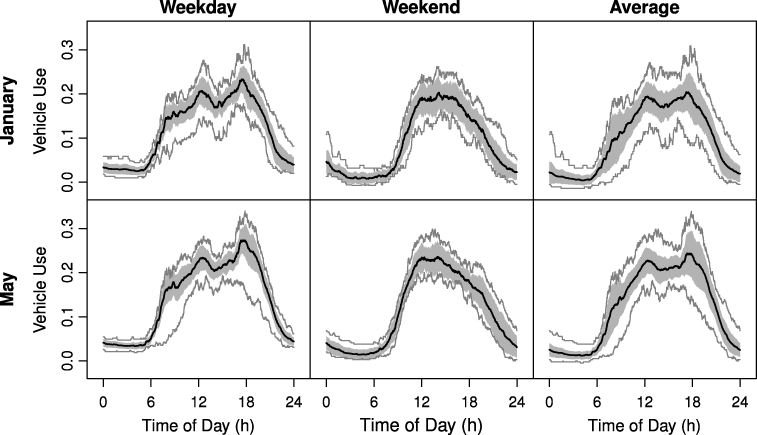
Figure 1. Weekday and weekend driving patterns differ significantly, regardless of the time of year, and averaging weekday and weekend data yields estimated vehicle use that is not reflective of either weekday or weekend patterns. The shaded gray area in each subplot shows the range of one standard deviation above and below the average. Gray lines indicate the maximum and minimum vehicle use values.
Download figure:
Standard image2.3. Results
Figure 1 shows for two months how vehicle use varies among weekdays, weekends and all days in the month. In each case, weekdays have two distinct local maxima, one around noon and another around 6 pm. In addition, weekdays show a rapid increase in vehicle use during the early morning hours, reflective of the morning commute to work, followed by a gradual increase towards peak use around midday. Weekend vehicle use is markedly different, characterized by use increasing later in the morning, a single peak around midday and a more gradual decrease in vehicle use throughout the afternoon and evening hours. The standard deviation of both the weekday and weekend data, shown as a gray area around the average, indicates that there is minimal variation in the magnitudes and timing of vehicle use within a month's weekdays and weekends. Though the timing and magnitude of the midday peak is similar for weekdays and weekends, averaging all the days of any month together yields a smoother use curve, associated with the lack of a rapid initial increase in use during the early morning hours and the absence of a second peak during the evening commute on weekend days. The mismatch between weekday and weekend vehicle use is also apparent from the standard deviation of the monthly averaged data, which does not follow the average line throughout the day. It is thus important to not use yearly or monthly averaged vehicle use patterns in V2G studies, as weekday and weekend vehicle use are markedly different.
Without further examination, the apparent conclusions from figure 1 could be misleading, particularly with respect to the separation of days of the week into weekdays and weekends. Figure 2 shows the average of each weekday over the course of the study period. As can be seen in these figures, the trends are similar regardless of the day of the week, supporting the earlier separation of data into weekday and weekend groups. It appears that there is a slight reduction in vehicle use throughout the first and last day of the work week, which could reflect alternative work schedules.
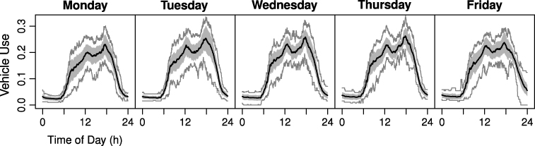
Figure 2. Comparing weekdays across all months in the study reveals that differences in vehicle use between weekdays are small.
Download figure:
Standard imageHaving separated the data into weekday and weekend groups, vehicle use was then compared across all the months in the study to determine whether use was affected by seasonal changes in weather or daylight hours. It was anticipated that meteorological conditions, both weather and the duration of daylight hours, could affect vehicle use in three primary ways: by encouraging or forcing individuals to stay home all day, to travel earlier or later than they otherwise would, and to slow down while driving, increasing congestion and travel times. These effects would appear in the data as a reduction in vehicle use throughout the day, a shift of or change in the duration of the daytime vehicle use period, and a widening and smoothing of the daytime vehicle use curve, respectively. A selection of months in the study, shown in figure 3, were examined for the potential appearance of these effects. These results do not show significant variation in the timing of peaks across months, indicating that weekday usage times are primarily affected by work or schedule requirements and not daylight or weather conditions. This indication is consistent with the minimal standard deviation that appears in figure 2. Widening, smoothing or shifting of daytime vehicle use periods does not appear to occur between months or within the data in each month. As noted in the US National Research Council's Transportation Research Board (TRB) Highway Capacity Manual, vehicle use patterns might be affected more dramatically in regions that experience severe winter weather conditions that make driving difficult [25].
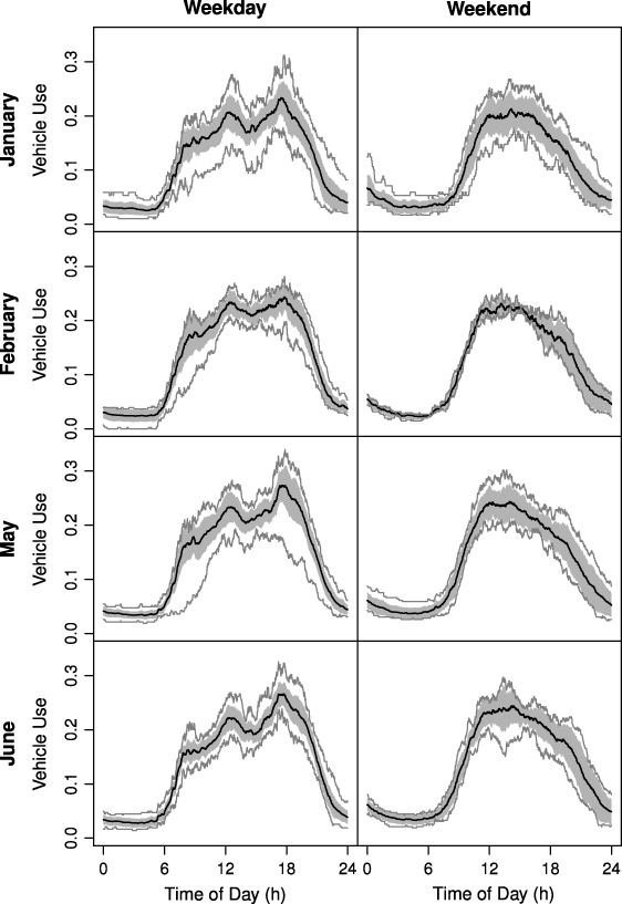
Figure 3. Trends in vehicle use on weekdays (left panel) or weekends (right panel) appear similar across months, suggesting that changes in weather or daylight hours are not significant factors.
Download figure:
Standard imageThere also exists the possibility of weather conditions impacting both renewable generation and vehicle use simultaneously. Such a common-mode change would require that a significant quantity of renewable generation be located near a concentration of BEVs such that they experience same weather conditions. (Large weather phenomena and natural disasters, such as hurricanes or earthquakes, are a notable exception.) In Texas, most wind generation is located far from major load centers and likely concentrations of BEVs. This geographic separation, as well as the lack of strong dependence of vehicle use on weather conditions allowed the combination of vehicle use data with wind generation and load data from the Electric Reliability Council of Texas (ERCOT).
Generally, the results in figures 1–3 are consistent with the TRB Highway Capacity Manual, in that urban vehicle use is relatively constant between weekdays but varies between weekdays and weekends, intra-day vehicle use is roughly bimodal, with peak use on weekdays in the afternoons around 5 or 6 pm, and variations in vehicle use between the same hours on different days of the month are small but not insignificant [25]. In addition to averaging the data to investigate patterns in vehicle use, various statistics on the study data were assessed to compare with national driving statistics, including the number of miles driven by each vehicle during the study period, the number of tours taken, and the number of days the vehicle was used. These data were largely consistent with the National Highway Transportation Survey (NHTS), conducted by the US Department of Transportation, except that annual vehicle mileage was lower in the PSRC study [30]. This difference in vehicle mileage could be a consequence of several factors, such as the geographic distribution of PSRC study participants or demographic differences between the NHTS and PSRC samples. Despite the difference in average annual vehicle miles traveled, comparison of the results against the TRB Highway Capacity Manual indicates that temporal trends observed in the vehicle use data are consistent with driving data collected in other municipalities [25]. This consistency indicates that while the PSRC data might underestimate volumes in other cities, the timing and trends in use are comparable, thus no further manipulation of the data was performed, as the primary focus of this work is on the temporal characteristics of vehicle use.
It should be noted that initially, BEV's usage patterns will likely differ from this data set. For example, two-car households with one EV might rearrange their vehicle use such that shorter trips are all taken using the EV and less-frequent, longer trips are completed using their other car. The details of how people will change their driving choices might be able to be estimated through close examination of driving patterns filtered with demographic parameters, along with forthcoming data on BEV use from early adopters, but this effort is subject to significant uncertainty and is outside the scope of this work. Further, it is anticipated that as BEVs become more widespread, purchasing moves beyond early adopters, and concerns like range anxiety are resolved through consumer education and improved public charging infrastructure, BEV use patterns will approach current vehicle use patterns in the general population.
BEV use patterns might also differ from current use patterns as a result of the financial incentives created by a V2G program. This effect is highly dependent on the magnitude of the revenue opportunities for vehicle owners; however, as the number of vehicles providing V2G increases and thus the importance of any behavior change increases, the revenue potential from providing V2G will probably diminish. Further study regarding the elasticity of departure time choice and the effect of increasing V2G participation on ancillary service capacity prices could illuminate the value of accounting for changes in driver behavior, but such analysis is outside the scope of this work.
3. Electricity market and battery availability analysis
3.1. Transformation of vehicle use into battery availability
In anticipation of comparison with data from ERCOT, vehicle use results discussed in section 2.3 were transformed to represent aggregate vehicle battery availability, or the total energy stored in the BEV fleet that is connected to the grid. This transformation requires modifying vehicle use, denoted by xt, to reflect battery charge depletion, Q, as a consequence of vehicle use during the day. Because BEV batteries have been aggregated for the entire fleet, an average distance driven can reasonably be substituted for a more complex distribution of tour lengths. The US average daily distance driven of 29 miles was used as a starting point for estimating charge depletion [26]. For a vehicle with a 24 kWh battery, such as the Nissan LEAF [27], if 40% charge depletion is assumed, 9.6 kWh would be depleted over the course of a tour. Assuming an approximate energy use of 0.34 kWh/mile [28, 29], 28 miles would be traversed in a tour, comparable to the US average daily driving distance.
For the example given, a 3.3 kW 240 V vehicle charger (EVSE) would require a minimum of 2.9 h (174 min) to recharge 9.6 kWh, and to allow for some deviation from the maximum charge rate, an average total recharge time, τ, of 3.2 h (192 min) was assumed. Implicit in this approach is the assumption that vehicles will be recharged only at the end of each tour. While it is possible that some drivers will have access to a charging station at work or while conducting business away from home, attempting to account for the potential availability of public or workplace EVSEs is outside the scope of this work.
Vehicle use is transformed into aggregate vehicle battery availability with equations (1)–(4). This analysis begins by equating the aggregate 'BEV storage use' fraction to the previously calculated 'vehicle use' fraction, xt, for all time t. As shown in equation (1), the difference between BEV storage use in each period t and the previous period t − 1 yields the variable δt. Each period in the model is 1 min in duration.

The total charge depleted (as a consequence of driving activity) from the batteries of vehicles completing tours and reconnecting to the grid in each period t is denoted by  , and is calculated as the charge depletion fraction, Q, of the change in BEV storage use, δt, as shown in equation (2). For example, if the BEV storage use fraction changes from 0.4 to 0.35 in a single period, δt will equal − 0.05 and the total charge depleted,
  , will be 0.02, assuming charge depletion, Q, is 40%. In periods where BEV storage use increases (vehicles are starting tours),
  is zero.

The quantity of charge restored in each period (minute),  , once vehicles' tours have ended, is described by equation (3). This quantity is simply the total battery depletion for period t that requires recharging,
  , divided by the number of periods (minutes) τ required for recharging.
Modifying BEV storage use, xt, with the parameters from equations (2) and (3) to reflect the effects of charge depletion yields 'adjusted BEV storage use', denoted by yt. In each period where BEV storage use decreases (δt is negative; vehicle tours are completed), yt is calculated by adding the charge depleted  from each of the last τ periods and then subtracting the fraction of the charge restored
  in each period, multiplied by the number of periods that have elapsed since the charge depletion event occurred. By including these two terms, adjusted BEV storage use thus reflects the state-of-charge of vehicles that have recently completed driving tours, at the time of their return (second term), as well as the time required to recharge their partially depleted batteries (third term). After τ periods, when the batteries of vehicles that completed tours in period t are fully charged, the latter two terms in equation (4) drop out, as indicated by the summation range on those terms.
The effect of charge depletion is especially evident in the evening hours when most tours end. Because of the charging time required, the cumulative effect of these charge-depleted BEVs completing their tours at the end of the day increases apparent vehicle use throughout the evening and early morning hours. It should be noted, as shown in figure 4, that partially depleted batteries can offer frequency regulation down, when a reduction in generation or an increase in load is needed to correct grid frequency, in addition to regulation up and spinning reserves. For later use with ERCOT data, the complement of charge depletion-adjusted BEV storage use was calculated following equation (5). This parameter, zt, is referred to here as 'battery availability'.

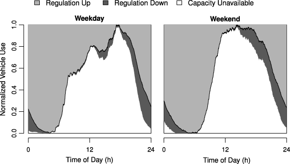
Figure 4. Normalized regulation up capacity is highest when most vehicles are stationary and fully charged in the early morning hours, before most tours begin, while regulation down capacity is highest in the evenings, when vehicles' tours are completed and their batteries have been partially depleted.
Download figure:
Standard image3.2. Comparison of ERCOT data and battery availability
Wind generation and electric load data from 2010 were obtained from ERCOT to compare with the vehicle use data described previously. These data were reported by ERCOT in 15 min intervals for each month, with generators grouped by fuel type, making wind generation and total load discernible. Data corresponding to the months missing from the PSRC data, July through October, were removed, and the remaining data were averaged in the same groups as vehicle use in preparation for subsequent comparisons.
Wind generation and electric load in ERCOT were compared with battery availability to determine whether battery availability and peaks in load were aligned. Net load, lt, which is load minus wind generation, was used for this comparison. Both battery availability and net load were normalized to fall between zero and one for the average weekday and average weekend of each month. The resulting parameter, at, that describes the comparison is denoted as 'availability–load alignment' and was calculated by multiplying battery availability and net load.

Peaks in the availability–load alignment curve reflect periods when vehicle batteries are most available to provide grid services and net load is relatively high. This approach assumes that neither the user nor the utility schedules charging of BEVs, but rather that vehicles will charge when owners plug them into an EVSE. As noted previously, it is assumed that charging will primarily take place at home, which is the terminus of most of the tours in the PSRC data. Depending on the extent to which net load and battery availability are aligned, BEVs might be available during peak demand hours when ancillary services are often crucial, or vehicle charging might not require widespread scheduling to ensure primarily nighttime charging. Figure 5 shows availability–load alignment for January. Representative of cooler months in Texas, wind generation comprises a greater portion of generation, and electric load is bimodal, with morning and evening peaks associated with residential activity and limited daylight hours. Alignment between battery availability and net load is best when availability–load alignment and net load are similar. Apart from overnight hours when net load is lowest, battery availability and net load in figure 5 show the greatest coincidence in the early morning hours, between 6 and 8 am, and in the late evening hours, after 9 pm. These periods of alignment arise from net load peaking when people are preparing to depart for work or errands in the morning, just before using their vehicles, and again when people complete their evening activities, having just used their vehicles for their last tour of the day.
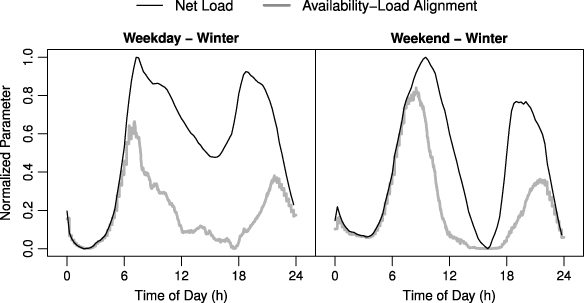
Figure 5. In the winter, hours of highest vehicle utilization in the morning and afternoon are bounded by periods of high electricity demand, before people leave home in the morning and after they arrive home in the evening, leading to strong alignment between availability and load during those hours.
Download figure:
Standard imageAs noted by many authors in the literature, in ERCOT, diurnal variations are present in both wind and load, and these variations change seasonally [4]. To examine seasonal variations, figure 6 shows battery availability, net load and availability–load alignment for June. Representative of hotter months in Texas, air conditioning loads yield high electricity demand during the afternoon and evening hours. Vehicle use shows a similar trend, with use peaking during the afternoon and evening hours. Because trends in vehicle use and net load are closely aligned, rising throughout the day, beginning around 6 am, and falling again in the evening, starting around 6 pm, the availability of vehicles to provide load shifting, peak shaving, or valuable ancillary services, is far more limited. Further, at times when vehicle use is lowest, net load is also near its minimum, and the potential value of V2G services is thus diminished.
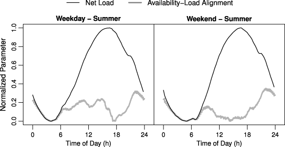
Figure 6. In the summer, battery availability is roughly the inverse of electricity load, leading to minimal alignment between the two parameters except on a limited basis midday and again in the late evening.
Download figure:
Standard image4. Conclusions
This study sought to assess the presence of patterns in vehicle use across various time intervals—within days, between days of the week and between months of the year. This research yielded two primary insights. First, diurnal driving patterns vary significantly between weekdays and weekends, and second, vehicles are often used during hours when grid services are in high demand, especially during the summer months, contrary to prior V2G studies. Examining GPS vehicle use data from the Puget Sound region revealed that weekdays and weekends show significantly different vehicle use profiles. Weekdays have three distinct periods—a rapid increase in vehicle use during the early morning hours, a midday peak and an afternoon peak. Weekends, on the other hand, have a single peak in vehicle use around midday, with lower use in the morning and late evening hours. Examination of the data for each day of the week revealed that variations within weekdays and weekends are comparatively minor. Identifying this difference between weekdays and weekends is crucial, as it indicates that V2G studies that use average driving profiles should be careful to not conflate weekday and weekend driving data, as doing so could result in under-prediction of vehicle usage, particularly in the early morning and late evening hours. The data also show that variation between months is limited, but the presence of seasonal variations could be a function of climate. In particular, in regions where winters are especially severe, limited daylight and poor weather conditions could restrict mobility, yielding lower overall vehicle use, and possibly a slight narrowing of the hours of high vehicle use. The households monitored in the PSRC study drove somewhat less than the average urban US household on an annualized basis, thus it is expected that these results and those for other regions differ only in the magnitudes of vehicle use.
This study also sought to compare the relationship between battery availability and net load, which is an indicator of periods when additional regulation is needed, to determine whether they are well matched. In ERCOT, battery availability appears to align best with net load during cooler months, when net load is bimodal and electricity use occurs primarily in the hours just before vehicles are used, between 6 and 8 am, and after tours are completed in the evening, beginning around 9 pm. Overnight, between those times, vehicles remain available to provide ancillary services while they recharge. In the summer, significant air conditioning loads in ERCOT yield a mismatch between net load and battery availability, suggesting V2G provision of grid services might be limited during those months. Given the regional dependence of wind (or other stochastic renewable) generation and electric load, and the potential for some variation in vehicle use between regions, it is important that researchers interested in performing V2G studies use regional data and, if possible, perform a long-term analysis to be able to account for seasonal variations in wind generation, electricity load and vehicle use. To that end, our future work will include more detailed modeling of seasonal V2G ancillary service capacity and will account for changes in ancillary service requirements to accommodate additional renewable generation.
Acknowledgments
The authors would like to thank the Electric Reliability Council of Texas, Bonneville Power Administration and the National Renewable Energy Laboratory for providing or making available the data facilitating this research. This work was supported by funding from the NSF Graduate Research Fellowship Program, Grant No. DGE-1110007.