
Abstract
The Kyoto Protocol compares greenhouse gas emissions (GHGs) using the global warming potential (GWP) with a 100 yr time-horizon. The GWP was developed, however, to illustrate the difficulties in comparing GHGs. In response, there have been many critiques of the GWP and several alternative emission metrics have been proposed. To date, there has been little focus on understanding the linkages between, and interpretations of, different emission metrics. We use an energy balance model to mathematically link the absolute GWP, absolute global temperature change potential (AGTP), absolute ocean heat perturbation (AOHP), and integrated AGTP. For pulse emissions, energy conservation requires that AOHP = AGWP − iAGTP/λ and hence AGWP and iAGTP are closely linked and converge as AOHP decays to zero. When normalizing the metrics with CO2 (GWP, GTP, and iGTP), we find that the iGTP and GWP are similar numerically for a wide range of GHGs and time-horizons, except for very short-lived species. The similarity between the iGTPX and GWPX depends on how well a pulse emission of CO2 can substitute for a pulse emission of X across a range of time-horizons. The ultimate choice of emission metric(s) and time-horizon(s) depends on policy objectives. To the extent that limiting integrated temperature change over a specific time-horizon is consistent with the broader objectives of climate policy, our analysis suggests that the GWP represents a relatively robust, transparent and policy-relevant emission metric.
Export citation and abstract BibTeX RIS
1. Introduction
Multicomponent climate mitigation policies, such as the United Nations Framework Convention on Climate Change (UNFCCC), need a method to compare the climate response of different emissions. Possibly based on an 'inadvertent consensus' between the IPCC and policymakers under the UNFCCC [1], the Kyoto Protocol compares emissions of the well-mixed greenhouse gases (GHGs) using the global warming potential (GWP) with many short-lived climate forcers excluded. The GWP was presented in the IPCC First Assessment Report (FAR) as a 'simple approach ... to illustrate the difficulties inherent in the concept, to illustrate the importance of some of the current gaps in understanding and to demonstrate the current range of uncertainties' [2]. To represent different climate responses, the IPCC presented three different time-horizons (20, 100 and 500 yr) 'as candidates for discussion [that] should not be considered as having any special significance' [2]. Given these careful waivers on the use of the GWP, it is perhaps surprising that the GWP, with a 100 yr time-horizon, has become entrenched as a robust method to compare GHGs.
Within the scientific community, there have been many critiques and discussions of the GWP concept [3–7]. A key issue is what the GWP represents in terms of a physical climate response [1, 8] and whether this is consistent with the objectives of climate policy [9, 10]. The GWP concept originated as a climate analogue of the ozone depletion potential (ODP) which compares the steady-state ozone depletion for a sustained emission relative to a reference gas [11]. Early development of the GWP considered the ratio of the steady-state forcing [12, 13] or temperature [14, 15] to a sustained emission. It was often assumed that for small perturbations temperature change was proportional to atmospheric abundance [13, 14]. This early literature suggests that the GWP was intended to represent steady-state temperature for a sustained emission; or equivalently, integrated temperature change for a pulse emission (see supporting information available at stacks.iop.org/ERL/6/044021/mmedia). During later developments, integrated forcing from a pulse emission was used [2, 16] and the direct link to temperature seems to have become lost.
In contrast to the ODP, a challenge with the GWP was the long-term response of the reference gas CO2, which did not reach a steady-state and required some arbitrary cut-off [14, 16] or time-horizon [2]. The IPCC FAR gave some tentative interpretations of the GWP depending on the time-horizon [2, 14]; a small time-horizon focuses on near term effects like rates of temperature change, while a long time-horizon focuses on cumulative impacts like sea level rise [2]. However, perhaps due to the similarity with the ODP, physical interpretations of the GWP often led to steady-state temperature change for a sustained emission (cf, [8]). Much later, O'Neill showed more concretely that the GWP can be interpreted as representing integrated steady-state temperature change for a pulse emission, if emissions are removed after the time-horizon [8]. The work of O'Neill, and analogies with the ODP, all lead to integrated temperature interpretations of the GWP, however we are unaware of attempts to consider this more directly or to interpret the non-steady-state behaviour of the GWP.
The motivation of this paper is to reinvigorate debate into the interpretation of, and relationship between, different emission metrics. The critiques of the GWP, a range of alternatives, and the likely development of a new climate regime, suggest that it is an opportune time to discuss alternative emission metrics. In particular, a more solid foundation for the relationship between the GWP and integrated temperature change can assist in assessing if the GWP is consistent with the broader objectives of climate policy. Our aim in this paper is to show the connections between the GWP and the integrated temperature change. We link various metrics via a single equation using an analytical energy balance model (EBM). This allows the emission metrics to be consistently compared and explored, and hence provides a foundation upon which to discuss alternative metrics.
2. Simple emission metrics
Simple emission metrics are usually derived for a pulse emission as pulses can characterize other emissions via a convolution [17]. The atmospheric response to a pulse emission is often represented by a sum of exponentials (SE) impulse response function,
giving the fraction of atmospheric component i that remains in the atmosphere after time t relative to a given reference system, often taken as constant current atmospheric conditions [18]. Most components have a single decay time (K = 1), though CO2 decays over multiple timescales and has a fraction that remains persistent in the atmosphere for millennia [19]. For small perturbations, the radiative forcing (RF) is usually assumed to develop linearly in proportion to the present radiative efficiency, Ai ,

The most common absolute emission metric is the absolute global warming potential (AGWP) which is the time-integrated RF,
As an alternative to the AGWP, the absolute global temperature change potential (AGTP) was developed [9, 10],

where RT is the temperature impulse response function to an instantaneous unit pulse of RF,
where the climate sensitivity λ = ∑k gk and hk are the decay times for the components of gk . RT can be thought of as a simple climate model based on a SE, but parameterized to emulate more complex climate models [20–22]. The rationale behind the AGTP is that it moves closer to the relevant response (temperature change), but at the expense of increased uncertainty [5, 9, 10, 23].
We formally define the integrated absolute global temperature change potential (iAGTP) as an integrated version of the AGTP,

The iAGTP has been discussed in relation to interpreting the GWP [8] and a similar metric has been proposed called the mean global temperature change potential (MGTP), where MGTP(t) = iAGTP(t)/t [24]. The AGTP for a sustained emission (e.g., [9, 25]) is equivalent to the iAGTP for a pulse emissions in a linear system (see supporting information available at stacks.iop.org/ERL/6/044021/mmedia).
It is common to normalize the absolute metrics to an index representing the climate response relative to a reference gas, usually taken as CO2,
where AM represents AGWP or AGTP leading to the global warming potential (GWP), global temperature change potential (GTP), or the integrated global temperature change potential (iGTP). Multiplying a normalized metric with the emission of component i, converts the emissions Ei into the equivalent emissions of CO2 (CO2-eq(t) = Mi (t)Ei ) that leads to the same climate response for the given metric [6, 8].
3. The relationship between alternative simple emission metrics
Metrics are often estimated with a SE impulse response function [9, 10, 18, 22] and a SE maps to a box-diffusion energy balance model (EBM) of the climate response [20]. Even though these EBMs are simplistic, they are still useful tools to understand the temporal behaviour of more complex models [20, 26, 27]. Consequently, we use an EBM as the analytical framework to compare emission metrics. Each 'box' in the EBM can be interpreted as ocean layers at different depths or different ocean timescales [20].
Consider an n-layer ocean EBM of the climate response to a forcing (cf [27]), where Ti is the temperature perturbation of layer i, ci is the specific heat capacity of layer i, and ki is the advective and diffusive heat flux into the next layer (cf [28]). The energy balance of the atmosphere–ocean mixed layer requires that the rate of change of the energy perturbation equals the energy added to the layer (forcing) minus the energy that is either radiated to space or transported to the next ocean layer,

where F1 is the RF at the top of the atmosphere and λ is the climate sensitivity which incorporates radiative feedbacks such as water vapour, clouds, sea ice and so on. In an intermediate ocean layer, the rate of change of the energy perturbation equals the energy transported from the layer above minus the energy transported to the layer below,

and in the bottom layer the rate of change of the energy perturbation equals the energy added to the layer from the layer above,

Adding all the layers together and assuming ci is constant gives the rate of change of the total energy perturbation of the ocean and equals the energy added to the ocean minus the energy radiated from the ocean back to space due to radiative feedbacks [27],
where E = ∑ci Ti is the total energy perturbation of the ocean and the energy content of each layer is Ei = ci Ti .
As we are interested in simple emission metrics, we force the EBM with a pulse emission. Integrating equation (11) for a pulse emission and assuming λ is constant leads to

where three metrics are included: the AGWP, the absolute ocean heat perturbation (AOHP) and the iAGTP. The AOHP can be linked to the AGTP

For a 1-layer EBM, AOHP = c1AGTP [9]. It has been argued that the ocean heat content (hence its perturbation, AOHP) is a better measure of the response of the climate system to anthropogenic forcing compared to surface temperature (e.g., [29, 30]).
These equations can be used to give a more physical representation of each absolute metric:
- AOHP(t) is the net energy perturbation in the system at t;
- AGTP(t) is the temperature perturbation of the atmosphere–ocean mixed layer at t;
- AGWP(t) is the cumulative energy added to the system from 0 to t;
- iAGTP(t)/λ is the cumulative energy radiated from the system back to space due to radiative feedbacks from 0 to t.
4. Comparison of GWP, GTP, and iGTP
We now explore the relationship between the various metrics, and in particular the iGTP and GWP, as a function of time-horizon for different species with different radiative efficiencies and adjustment times. Using SE for the atmospheric and temperature responses to a unit impulse, we took analytical expressions for AGWP and AGTP, hence GWP and GTP from an earlier study [5] and by integrating the AGTP we derived analytical expressions for iAGTP and iGTP (see supporting information available at stacks.iop.org/ERL/6/044021/mmedia). The AOHP is calculated from equation (12). The radiative efficiencies and adjustment times are from earlier work [5]. We parameterize the EBM using the SE temperature response from the Hadley model [22], though we perform a sensitivity analysis with different parameterizations.
We compare four species, in addition to CO2, to demonstrate our results. CO2 has multiple decay times (1.2, 18.5, 172.9 yr) [18] and does not converge to zero at infinity creating problems in metric specification [8]. We chose species with adjustment times covering five orders of magnitude: a very short adjustment time (black carbon, BC, 0.02 yr or 1 week), short adjustment time (methane, CH4, 12 yr including indirect effects), medium adjustment time (nitrous oxide, N2O, 114 yr), and long adjustment time (sulfur hexafluoride, SF6, 3200 yr). Figure SI1 available at stacks.iop.org/ERL/6/044021/mmedia shows the atmospheric response of these species together with the components of the response for CO2, demonstrating that the decay profile of CO2 has components that approximate the atmospheric decay of CH4 (18.5 yr CO2, 12 yr CH4) and N2O (172.9 yr, 114 yr). All our figures use a log scale for time from 0.01 to 10 000 yr to capture the temporal evolution of both BC and SF6, though we recognize that emission metrics and climate models are unreliable at these extreme times. We also recognize that for very short- and short-lived species the forcing and response is regional [31, 32] and thus assuming a global forcing and response is idealized.
4.1. Temporal evolution of AGWP, AGTP, iAGTP and AOHP
Figure 1 shows the absolute metric values (AGWP, AGTP, iAGTP and AOHP) as a function of time for pulse emissions. For the species shown, energy is added to the system via the RF with a single adjustment time. The RF eventually decays to zero, independent of the climate model, and the cumulative energy added to the system is AGWP. Whilst the RF is in place, energy is continually transported into the ocean layers (AOHP and c1AGTP increase). As the RF decays back to zero, the energy in the system (AOHP) also decays back to zero as energy is radiated back to space (iAGTP/λ) at different timescales dependent on the climate system (figure SI2 available at stacks.iop.org/ERL/6/044021/mmedia). The AOHP eventually decays to zero, and to retain energy balance, the energy that is radiated back to space (iAGTP/λ) eventually equals the energy that was added (AGWP), equation (12).
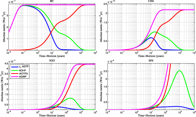
Figure 1. The absolute metric values for BC, CH4, N2O and SF6 showing the relationship between AOHP and c1AGTP in addition to how iAGTP/λ converges to AGWP depending on the atmospheric adjustment times (cf figure SI1 available at stacks.iop.org/ERL/6/044021/mmedia). In this figure all the metrics have the same unit.
Download figure:
Standard imageWhen the RF is present, energy is continually added to the first layer, but the energy is lost from the first layer in two directions (equation (8)): (1) back to space dependent on T1/λ, and (2) into the deeper ocean dependent on the temperature gradient k1(T1 − T2). The ocean acts to increase the duration of the energy release back to space [27, 33]. The first component, T1/λ, dictates how energy is lost from the system, and due to the inertia in the ocean, energy remains in the system (AOHP) even after the forcing decays to zero. The second component, k1(T1 − T2), puts energy into the deeper ocean dependent on the temperature gradient. Even for the very short-lived BC, energy moves into the deep ocean (figure 1). In many climate model parameterizations, T1/λ and k1(T1 − T2) are comparable in magnitude (table SI1 available at stacks.iop.org/ERL/6/044021/mmedia).
As the RF decays towards zero, the energy perturbation remaining in the ocean causes a persistent temperature response in the top layer. The slowest timescale of the ocean, hn , usually the deepest layer, dictates the duration of the temperature persistence. The persistence is relatively longer for species with a short adjustment time. As an example, even though BC has an atmospheric adjustment time of around 1 week and CH4 12 yr, the duration of the temperature perturbation following a pulse emission is still more than 500 yr for both in the EBM used here. When energy moves from the deep ocean through the surface layer and back to space, the surface temperature is approximately constant (figures SI3–4 available at stacks.iop.org/ERL/6/044021/mmedia). Hence, the flux into the top layer from the deep ocean k1(T1 − T2) is approximately equal to the flux to space T1/λ. Consequently, the top layer does not accumulate more energy when energy is transported from the deep ocean back to space (figure 1). The temperature in the top layer only decreases when the energy in the top layer is reduced.
The relative values of the parameters, hence timescales, used to replicate the climate system only change when different processes occur and do not change the qualitative conclusions. The absolute metric values in figure 1 depend on the species adjustment time and the timescales of the climate response. Energy is added to the system with the adjustment time of the species τX(F), while energy is radiated back to space (Ti /λ) with the timescales of the EBM modulated by the species' adjustment time (equations (SI9) and (SI10) available at stacks.iop.org/ERL/6/044021/mmedia). For the two layered EBM used here, three situations can arise: (1) τX < h1, (2) h1 < τX < h2, and (3) h2 < τX. In the first case (BC) the timescales of the EBM (h1 and h2) dominate AGTP and hence iAGTP, in the second case (CH4 and N2O) τX and h2 dominate, and in the third case (SF6) τX dominates (see figures SI2 available at stacks.iop.org/ERL/6/044021/mmedia). The unevenness of the responses to a pulse emission in figure 1 is due to the interaction of the timescales of the forcing and the climate system.
4.2. The relationship between iGTP and GWP
Based on equation (12), iAGTP/λ eventually converges to AGWP since the AOHP will progressively become relatively small in relation to AGWP and iAGTP/λ. However, this does not necessarily imply that the normalized metric iGTP converges to GWP, or if they converge, it does not imply it happens at the same timescale. This distinction is important since the normalized metrics compare the response of the system to a forcing by X with the forcing due to a CO2-equivalent forcing designed to mimic the response of X. The difference between iGTP and GWP requires understanding how the system responds to a forcing of X compared to a CO2-equivalent forcing, and potentially, how these differences interact with the timescales of the climate system.
Figure 2 shows the relationship between iGTP and GWP by plotting them together with their relative difference, and table 1 shows the metric values for common time-horizons. The metric values are within about 10%, except for BC. The metric values will eventually converge due to the long-term divergence of iAGTPCO2. Qualitatively, the largest differences occur around the time constants of the climate system and atmospheric adjustment time of the different species dependent on the relationships between h1, h2, and τX as described earlier. In the case of BC, large differences occur at early times and persist much longer than for the adjustment time of BC.
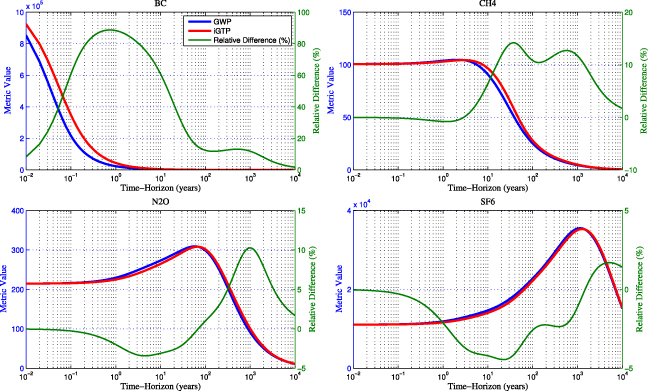
Figure 2. A comparison of iGTP, GWP, (left axes) and their relative difference (right axes) for BC, CH4, N2O and SF6 showing that iGTP and GWP are numerically similar for a wide range of time-horizons, except for the case of BC.
Download figure:
Standard imageTable 1. The GWP, iGTP and GTP values for time-horizons of 20, 50, 100 and 500 yr. The iGTP and GWP become more similar for species with greater adjustment times. The GTP and GWP are generally dissimilar, except when CO2 is able to reproduce the forcing profile of the species, such as for N2O (figure 3).
| TH | GWP | iGTP | iGTP/GWP | GTP | GTP/GWP |
|---|---|---|---|---|---|
| Black carbon (adjustment time, 0.02 yr) | |||||
| 20 | 1 595 | 2 254 | 1.41 | 462 | 0.29 |
| 50 | 770 | 913 | 1.19 | 77 | 0.10 |
| 100 | 453 | 510 | 1.12 | 64 | 0.14 |
| 500 | 138 | 156 | 1.13 | 29 | 0.21 |
| Methane (adjustment time, 12 yr) | |||||
| 20 | 72 | 81 | 1.12 | 57 | 0.80 |
| 50 | 42 | 48 | 1.14 | 12 | 0.29 |
| 100 | 25 | 28 | 1.11 | 3.8 | 0.15 |
| 500 | 7.7 | 9 | 1.13 | 1.7 | 0.21 |
| Nitrous oxide (adjustment time, 114 yr) | |||||
| 20 | 290 | 282 | 0.97 | 303 | 1.05 |
| 50 | 308 | 306 | 0.99 | 322 | 1.05 |
| 100 | 299 | 302 | 1.01 | 265 | 0.89 |
| 500 | 154 | 165 | 1.08 | 51 | 0.33 |
| Sulfur hexafluoride (adjustment time, 3200 yr) | |||||
| 20 | 16 228 | 15 507 | 0.96 | 17 485 | 1.08 |
| 50 | 19 485 | 18 760 | 0.96 | 23 331 | 1.20 |
| 100 | 22 767 | 22 180 | 0.97 | 27 948 | 1.23 |
| 500 | 32 544 | 31 798 | 0.98 | 38 659 | 1.19 |
The numerical difference between the metric values can be expressed as
This can be expressed equivalently in terms of AOHP by using equation (12) and noting that by definition AGWPX = GWPX × AGWPCO2. The denominator (iAGTPCO2) is always positive and grows towards infinity with time and thus it only acts to reduce the magnitude of the difference as time progresses; hence GWP and iGTP will converge with time since iAGTPCO2 diverges.
At smaller times before iAGTPCO2 dominates the difference, the numerator on the right-hand side of equation (14) dictates the size of the difference between GWP and iGTP,

which shows that the difference DX depends on how

interacts with the timescales of the climate system given by RT . The second term on the right-hand side of equation (17) is the actual forcing of X, while the first term can be defined as the 'CO2 equivalent forcing of X with respect to the GWP',

where t is the fixed time-horizon and u is variable. Integrating equation (17) with respect to u, and evaluating at t, replicates the AGWP by definition, AGWPX = GWPX × AGWPCO2.
The similarity between different metrics, therefore, depends on how well RFX(CO2) can substitute RFX for the given t and how these differences interact with the timescales of the climate model. Figure 3 shows RFX and RFX(CO2) for a pulse emission and different time-horizons. Each dotted curve, RFX(CO2), is the forcing with the same normalized response curve as CO2 but scaled by GWPX. When RFX(CO2) is integrated to the given time-horizon, black circles, it leads to equal values of AGWPX and AGWPX(CO2). The figure shows that for most species and time-horizons, CO2 is unable to represent the temporal behaviour of the forcing of the different species even though it leads to the same AGWP. More mathematically, RFX and RFX(CO2) have by definition equal integrals, but they have different forcing pathways to arrive at those integrals. RFX(CO2)will at some times overstate RFX and at other times understate RFX, but these differences balance leading to equal integrals at the chosen time-horizon. In the most extreme case of BC, RFX(CO2) always overstates the RFX for timescales greater than 0.1 yr. For the other species, the times that RFX(CO2) overstates and understates RFX is more evenly distributed over the timescales of the climate system. It is the differences in RFX(CO2) and RFX that leads to the differences in iGTP and GWP.
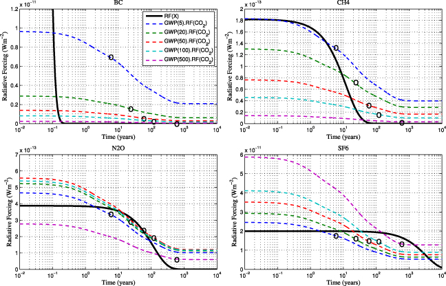
Figure 3. The RF for a pulse emissions of X, RF(X), and a CO2-eq emission of X for different fixed time-horizons (TH), GWP(X) × RF(CO2). The CO2-eq forcing, as a function of time, reproduces the AGWP values (integral of the curves) for the given time-horizon (black circles) despite the potentially large differences between RF(X) and GWP(X) × RF(CO2).
Download figure:
Standard imageCO2 is characterized by several adjustment times (figure SI1 available at stacks.iop.org/ERL/6/044021/mmedia), all of which, together, must represent the response of a species with a single adjustment time. CO2 is unable to reproduce the very short adjustment time of BC, and to compensate for this, RFX(CO2) has a relatively small but persistent forcing profile. The different forcing profiles leads to AOHPX(CO2) being higher than AOHPX (figure SI2 available at stacks.iop.org/ERL/6/044021/mmedia), and hence more energy is radiated back to space or transported to the deeper ocean for the CO2-eq forcing. These two fluxes out of the first layer explain the difference between GWP and iGTP (figure 2). The same issues arise for CH4, but since the CO2-eq forcing is more similar to the pulse of CH4, the differences are not as pronounced and hence GWP and iGTP differ less for CH4. In the case of N2O, RFX(CO2) represents a pulse of N2O reasonably well, leading to a smaller relative difference in GWP and iGTP (figure 2). The small difference between RFX and RFX(CO2) also means that GWP and GTP are similar for N2O (table 1). In the case of BC, CH4, and N2O, when the time-horizon is greater than the adjustment time of the species, the CO2-eq forcing does not decay to zero (figure 3) and continually puts more energy into the system leading to a larger AOHPX(CO2) at these times (figure SI2 available at stacks.iop.org/ERL/6/044021/mmedia). SF6 has a longer adjustment time than CO2 and hence SF6 initially puts more energy into the system, though this changes as the time-horizon exceeds the adjustment time of SF6. In all cases, since RCO2 does not decay to zero, iAGTPCO2 eventually dominates the difference between GWP and iGTP and cancels any persistent differences in AOHP. Hence, for sufficiently long time-horizons iGTP converges to GWP. Thus, the differences between the iGTP and GWP for a pulse emission of X and a CO2-eq pulse emission of X depend on how well CO2 can represent the adjustment times of X. Additional simulations showed that different timescales in the background climate system do not change these conclusions, the timescales only shift when differences occur.
To determine whether our findings are dependent on the timescales of RFCO2, we repeated our analysis with different reference gases. First, we artificially modified RFCO2 to include a component with short adjustment times similar to BC. This did not improve CO2 as a reference gas since CO2 has a variety of adjustment times (figure SI1 available at stacks.iop.org/ERL/6/044021/mmedia), and RFX(CO2) must include a compensation across all these adjustment times. Second, we used reference gases with a single adjustment time, such as BC, CH4, N2O and SF6, and the same issues persist as the reference gas may be able to represent one adjustment time well, but not others. This highlights that selecting a reference gas to cover species with many order of magnitude differences in adjustment times is difficult. This suggests the use of multi-basket approaches [34, 35], where each basket has a different reference gas.
To ensure our results are robust and assess uncertainties, we repeated our analysis for a variety of SE impulse response functions in the literature covering 1-, 2- and 3-layer models [9, 20, 21, 28], table SI1 (available at stacks.iop.org/ERL/6/044021/mmedia). We found the results qualitatively robust across the different IRFs, despite some variations due to the different timescales in each IRF. We found that the iGTP values are relatively robust (low variation) despite large variations in response functions (figure SI6 available at stacks.iop.org/ERL/6/044021/mmedia). We found larger variations in GTP values than iGTP (figure SI7 available at stacks.iop.org/ERL/6/044021/mmedia), and this could be expected since GTP is an instantaneous metric and iGTP is integrated. Gillett and Matthews [24] proposed a similar metric MGTP(t) = iAGTP(t)/t that when normalized to CO2 shows similar numerical values to the GWP when t = 100 yr. Jacobson [25] develop a metric 'surface temperature response per unit continuous emissions' (STRE) which is equivalent to the iAGTP for a pulse emission (see supporting information available at stacks.iop.org/ERL/6/044021/mmedia), and finds similar values to GWP. Based on these assessments, we believe that the similarity between iGTP and GWP is likely to be robust across a range of parameter values and climate models. Though, further modelling would be required to confirm these observations.
4.3. Comparison with O'Neill [8]
O'Neill [8] gave a well-defined interpretation for the AGWP in terms of the iAGTP, however, under a restrictive set of assumptions. He assumed that the emissions did not affect RF beyond the time-horizon, that is, emissions went to zero at the time-horizon. Next, O'Neill showed that continuing the integration to infinity leads to equal integrated temperatures. This is a direct consequence of the energy balance in equation (12). To see this, suppose that  is the integrated forcing for a pulse emission of X from time zero to TH, and
  is the equivalent for the CO2-equivalent forcing. It follows that

and likewise for CO2. Since the ocean does not permanently store energy, and the emissions are truncated at TH, then it follows that AOHPX TH converges to zero as time progresses and thus,

Since emissions are removed after TH,  also converges to zero. By construction,
  , and hence it follows directly by energy conservation that,
  .
.
5. Discussion
We used a layered EBM of the climate system to link the metrics AGWP, iAGTP, AGTP and AOHP via one equation to allow a transparent discussion of emission metrics. The similarity between AGWP and iAGTP is since they measure approximately the same physical quantity; the AGWP represents the total energy added to the system and the iAGTP/λ the total energy lost. Since the energy perturbation currently in the system (AOHP) eventually tends to zero for a pulse emission, then iAGTP/λ must converge to AGWP by energy conservation. We found that the GWP and iGTP were similar numerically to within about 10% for a wide range of species and time-horizons, except for species with very short adjustment times such as BC. Differences between GWP and iGTP arise when CO2 is unable to adequately substitute the temporal behaviour of the RF of the different species, as highlighted in the case of BC. It is expected that the GWP and GTP would be different as one is an instantaneous property (GTP) and the other is an integrated property of the system (GWP); that is, for the GTP the pathway of the forcing is most important while for GWP the integral is most important. The parameters used to model the climate system do not change the qualitative conclusions, only the time at which the differences occur.
Whilst this article has focused primarily on the GWP and iGTP, we do not wish to place any particular preference to one metric over another. Metrics require a variety of value-based and scientific choices [6, 36], and the value-based judgements are beyond the scope of this paper. In terms of the scientific choices, a continuing debate in the emission metric literature is the trade-off between simple metrics (like the GWP, GTP and iGTP) and the use of more complex metrics [3, 4, 8]. Since metrics such as the GTP and iGTP include a climate model, it would be expected that they have a greater uncertainty; however, we find that the instantaneous metric GTP is more sensitive to the climate model than the integrated metric iGTP (see figures SI6–7 available at stacks.iop.org/ERL/6/044021/mmedia). Despite the potential limitations of the GWP, an advantage is that it is transparent and only requires models of the atmospheric response of different components without the need for a climate model (unless including feedbacks) and hence it would be expected to have less uncertainty than the GTP or iGTP. The GWP is often placed at the 'forcing step' in the cause effect chain [6], however, its relationship to the iGTP suggests that it should be interpreted in the context of integrated temperature. The iGTP interpretation of the GWP is also consistent with its early development [14, 15]. To the extent that limiting integrated temperature change over a specific time-horizon is consistent with the broader objectives of climate policy, our analysis suggests that the GWP represents a relatively robust, transparent and policy-relevant emission metric.
Acknowledgments
This work was partially funded by the Norwegian Research Council project Climate and health impacts of Short Lived Atmospheric Components (SLAC) and the US Federal Aviation Administration project Aviation Climate Change Research Initiative (ACCRI). We thank the following for valuable input and comments: Bill Collins, Brian O'Neill and Keith Shine. Two reviewers provided valuable comments.