

Abstract
While changes in temperature and precipitation extremes are evident, their influence on crop yield variability remains unclear. Here we present a global analysis detecting yield variability change and attributing it to recent climate change using spatially-explicit global data sets of historical yields and an agro-climatic index based on daily weather data. The agro-climatic index used here is the sum of effective global radiation intercepted by the crop canopy during the yield formation stage that includes thresholds for extreme temperatures and extreme soil moisture deficit. Results show that year-to-year variations in yields of maize, soybean, rice and wheat in 1981–2010 significantly decreased in 19%–33% of the global harvested area with varying extent of area by crop. However, in 9%–22% of harvested area, significant increase in yield variability was detected. Major crop-producing regions with increased yield variability include maize and soybean in Argentina and Northeast China, rice in Indonesia and Southern China, and wheat in Australia, France and Ukraine. Examples of relatively food-insecure regions with increased yield variability are maize in Kenya and Tanzania and rice in Bangladesh and Myanmar. On a global scale, over 21% of the yield variability change could be explained by the change in variability of the agro-climatic index. More specifically, the change in variability of temperatures exceeding the optimal range for yield formation was more important in explaining the yield variability change than other abiotic stresses, such as temperature below the optimal range for yield formation and soil water deficit. Our findings show that while a decrease in yield variability is the main trend worldwide across crops, yields in some regions of the world have become more unstable, suggesting the need for long-term global yield monitoring and a better understanding of the contributions of technology, management, policy and climate to ongoing yield variability change.
Export citation and abstract BibTeX RIS

Original content from this work may be used under the terms of the Creative Commons Attribution 3.0 licence. Any further distribution of this work must maintain attribution to the author(s) and the title of the work, journal citation and DOI.
1. Introduction
Climate extremes are a key driver affecting food production and food-export policy, as exemplified by the 2012 drought in the United States and the 2010–2011 Russian wheat embargo. Given the increased volatility of commodity markets [1] and the rising incidence of climate extremes [2, 3], food price spikes may become more prevalent in coming decades [4–6]. Because consumers, including the poor in many countries, are increasingly dependent on food imports [4], the rising incidence of climate extremes and changing variability in yield, production and export prices in the world's major food producers are of concern for national governments and commercial entities in import-dependent countries [4, 7, 8].
In the last few years, some global studies analyzing the yield impacts due to historical and future temperature extremes from the crop exposure to high temperatures during key growth stages (e.g., flowering) have become available [9–11]. A study [12] analyzed global climate–crop relationship, including monthly temperature and precipitation extremes. A few regional studies have explicitly projected future yield variability changes [13, 14]. While these analyses have provided new insights, we know little about how changes in daily temperature and precipitation extremes in the last few decades have influenced historical yield variability.
We conducted a global analysis to detect changes in yield variability of maize, soybean, rice and wheat and attribute them to climate change using recently developed spatially-explicit global data sets of historical yields [15] and daily weather [16]. These four crops are the principal cereal and legume crops worldwide, providing nearly 60% of all calories produced on croplands [17]. The main question we addressed here was: have recent changes in daily temperature and precipitation extremes had a measurable influence on yield variability? Previous work on yield variability change and its attribution either focused on smaller geographical regions [18–20] or conducted global analysis that lacked subnational information [21]. Moreover, few global studies dealt with daily temperature and precipitation extremes. We expect that the agro-climatic index approach adopted in this study, which is based on more process-based understanding than previous approaches, and using daily weather inputs, will provide new insights into the historical impacts of climate change on yield variability.
2. Methods
2.1. Crop yield data
The 30 year long (1981–2010) 1.125° annual yield time series of maize, soybean, rice and wheat obtained from the global data set of historical yields [15] and its update were used. The data set includes two different types of grid-cell yields—uniformly disaggregated subnational yield statistics (or aggregated for small administrative units) reported by governmental agencies (available for 23 countries) and hybrid satellite-statistics yield estimates. We mainly used the hybrid yield estimates for this study, but our overall conclusions were tested using the two types of the data. This approach is important because the hybrid yield estimates are modeled data and have uncertainties associated with errors in the underlying satellite-derived vegetation index and use of time-constant information on harvested area, crop calendar and cropping systems. This data set provides yield estimates for a substantial portion of the global cropland. However, data in a number of locations are not available due to the lack of crop calendar information that is an essential input for the hybrid yield estimation procedure [15].
Two different yield de-trending methods were adopted in this study: the running mean (RM) yield which assumed that five-year RM yield (year t − 2 to t + 2) represented normal yield and a deviation of yield from the normal indicated yield anomaly, according to [22]; and first-difference (FD) of yields which assumed that normal yield was represented by three-year RM yield (year t − 3 to t − 1) and FD of yields indicated yield anomaly, as in [21] and [23]. In both methods, yield anomaly was expressed as a percent relative to normal yield, as in previous studies [18, 19, 21–23].
To characterize yield variability change, two different measures of variability change were used: the slope of a linear regression line fitted to a nine-year running window time series of the standard deviation (SD) of yield anomalies (Slp), according to [18]; and the ratio of SD of yield anomalies for the later years (1996–2010) relative to that for the earlier years (1981–1995) (SDr). The statistical significance of yield variability change was tested using the bootstrap method [24]. Therefore, four different method–measure combinations, RM–Slp, RM–SDr, FD–Slp and FD–SDr, were used to account for the methodological uncertainty in the detection of yield variability change. More detailed descriptions for yield data processing are available in section S1 in the supplementary information.
2.2. Agro-climatic index
2.2.1. Overview of the index
An agro-climatic index—annual time series of the sum of effective radiation intercepted by the crop canopy during the yield formation stage that includes thresholds for extreme temperatures and extreme soil moisture deficit—was used to describe the influences of irrigation and day-to-day weather fluctuation on the length and timing of the yield formation stage and potential yield (figure 1). Daily maximum and minimum temperature, potential and actual evapotranspiration rates, snow cover, and global radiation during the yield formation stage were input data to calculate the index. Abiotic stresses that influence potential yield, such as temperatures above and below the optimal range for yield formation and soil water deficit during the yield formation stage, were also incorporated into the index calculation.
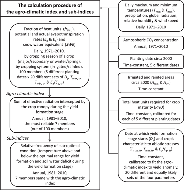
Figure 1. Schematic illustrating the calculation procedure of the agro-climatic index and sub-indices.
Download figure:
Standard image High-resolution image2.2.2. Calculation of the index
Modeled crop phenology, potential leaf area and canopy height calculated based on formulations in the Soil and Water Assessment Tool [25] were used as the inputs to the index calculation procedure (see sections S2.1 and S2.2 for details). Potential evapotranspiration rate was estimated using a variant of Penman–Monteith method that accounts for the influence of increasing atmospheric carbon dioxide concentration (CO2) on leaf conductance [25]. Actual evapotranspiration rate was derived based on the potential evapotranspiration rate and available root-zone soil moisture computed by the soil water balance model [26] coupled with the snow cover model [27]. These physical and biophysical processes were simulated at a daily time step. A 11-year long (1970–1980) soil moisture spin-up simulation was conducted before using the simulated outputs for the index calculation. Then index value was computed by cropping season of a crop (major and secondary or winter and spring) and by cropping system (rainfed and irrigated) and averaged to derive a grid-cell mean value of the index using the grid-cell extent of irrigated and rainfed areas [28] and the share of production by cropping season [29] as the weights.
When calculating the annual index time series, we assumed five different planting dates to take into account the uncertainty of index value due to different management conditions (figure 1, see also section S2.3). Furthermore, we used the Bayesian calibration technique that estimates parameter values in a probabilistic manner (i.e., the posterior distribution of a parameter) to represent the uncertainty of parameter values given the data. This characteristic of the Bayesian calibration technique is useful to explicitly incorporate parametric uncertainty into the index calculation. Each posterior distribution of the four parameters (Dy, Tmax, tr, Tmin, tr and Ea/Ep, tr in figure 1; see sections S2.1 and S2.4 for details) was estimated separately for each grid cell by fitting the index value to the yield anomaly in the calibration period (1989–2001). Then, for each planting date, we estimated 20 different ensembles of the index values based on different and equally likely sets of the parameter values generated from the posterior distributions. The index time series was separately calculated for each member of the ensemble. As shown in figure 1, we used the seven most reliable members among the 100 members consisting of five different planting dates and 20 different parameter sets (so planting date could vary among the seven members) for further analysis. Because the selection of members was assumed to be a part of the calibration procedure, the selection was based on the correlation coefficient between the yield anomaly and the index in the calibration period. The basic assumption behind this model selection procedure is that the selected seven members best represent local management and technological conditions (as done in [14]).
2.2.3. Comparing yield variability change with change in the variability of the index
As with yield, we calculated two measures of variability change (SDr and Slp) for the index for comparison with yield variability change. For a consistent comparison, FD of the index was compared with yield variability change derived based on FD de-trending method. Index anomaly from the 1981–2010 long-term mean was used to compare against yield variability change derived based on RM de-trending method. The bootstrap method [24] was used for the significance test of index variability change, as with yield, but for each member. We assumed that change in the variability of agro-climatic condition (indicated by the index) was consistent only when over two-third (>5) of the seven members showed significant results with the same direction of change.
2.2.4. Sub-indices
In addition to the main index mentioned above, we separately computed three sub-indices using the same inputs to the index calculation (figure 1): (1) the percentage of days with temperature above the optimal range for yield formation during the yield formation stage (that is, relative frequency), (2) relative frequency of temperatures below the optimal range for yield formation, and (3) soil water deficit during the yield formation stage. Then changes in the variability of these sub-indices were calculated in the same manner as already noted for the main index. A day with temperature above and below the optimal range for yield formation was defined based on daily maximum and minimum temperature, respectively, whereas a day with soil water deficit was based on the fraction of actual-potential evapotranspiration rates (see section S2.1).
3. Results
3.1. Historical changes in yield variability
Our analysis of yield variability change for the last 30 years shows that yield variability in 19%–33% of the global harvested area significantly decreased with varying extent of area by crop (p < 0.05, two-tailed test, figure 2). In contrast, yield variability in 9%–22% of the harvested area significantly increased. For maize and soybean, the extent of area with decreased yield variability was 2–3 times the area with increased yield variability. However, for wheat, the areas with contrasting changes were comparable. These results were based on a specific method referred to as RM–Slp, but similar results were obtained using three different and equivalent methods except for rice (FD–SDr, FD–Slp and RM–SDr, figures S1 and S2). For rice, RM–Slp method found that the areas with contrasting changes were almost comparable, whereas the other methods found that rice yield variability decreased in many more areas than it increased (figures S1 and S2). While we first presented the results from RM–Slp method for explanatory purpose, all methods are equivalent and consistent results across different methods is likely more robust than a result derived from any single method.

Figure 2. Yield variability change during 1981–2010 for four crops. Data derived from RM–Slp method and the hybrid yield estimates are presented. The significance level of variability change was set to be 5% (two-tailed test; and the bootstrap replication of 1000 times). The sample size per grid cell was ∼18 because the nine-year running window was applied to the five-year-running-mean-derived 26 yield anomalies in the 30-year period. The analysis was performed only when ten or more samples of the nine-year-running-window-derived standard deviation of yield anomalies were available. The pie diagrams indicate the percentages of global harvested area in the colored areas, normalized to the global harvested area in 2000.
Download figure:
Standard image High-resolution imageThe locations of increased yield variability varies by crop, but a relatively consistent signal of increased yield variability across these crops was found for Southern Europe, Northeast China and southeastern part of South America (figures S1 and S2). In addition, increased wheat yield variability in Australia and Eastern Europe is prominent. A relatively consistent signal of decreased yield variability emerged in the United States and Eastern China. Importantly, these changes in yield variability were robust when using different global yield products—our hybrid satellite-statistics dataset [15] or those derived from subnational yield statistics, although the sign (decrease or increase) and amplitude of yield variability change at a grid-cell level varied by data source to some degree (figure S3).
3.2. Yield variability changes versus changes in the variability of agro-climatic condition
We quantified the major characteristics of yield variability change using a nine-year running window time series of the SD of yield anomalies, as in previous work [18, 19]. We then assumed that the agro-climatic index could reliably capture yield variability change for a given location and crop when the correlation coefficient calculated between the SD time series of yield anomalies and the SD time series of the index was significant (p < 0.05, two-tailed test) and the significant results were consistent across over two-third (>5) of the seven members. This condition is important to ensure the skill of the index in capturing major characteristics of yield variability change.
When RM de-trending method was used, the index reliably captured yield variability change in 67%–70% of the harvested area (figure 3). Nearly identical results were obtained by other de-trending methods (figure S4). However, in 5%–11% of the harvested area, either (or all) of the ensemble members showed insignificant correlation with yield variability and therefore assumed less reliable (figures 3 and S4). In the remaining 21%–30% of the harvested area, no yield data or a limited number of yield data was available. Those areas were therefore discarded from further analysis. Consequently, this study offers a global assessment covering over 60% of the harvested area worldwide (figures 3 and S4).

Figure 3. Locations where the major characteristics of yield variability change could be reliably explained by the agro-climatic index. Data derived from RM yield de-trending method and hybrid yield estimates are presented. The nine-year running window time series of the standard deviation of yield anomalies and those of the index were compared. If the correlation coefficient was significant at the 5% level (two-tailed test, the bootstrap replication of 1000 times) and the significant results were consistent across over two-third (>5) of the seven members then the index was assumed reliable. Otherwise, the index was assumed less reliable. The sample size per grid cell and member was ∼18 because the nine-year running window was applied to the five-year-running-mean-derived 26 yield anomalies in the 30-year period. The analysis was performed only when ten or more samples of the nine-year-running-window-derived SD of yield anomalies were available. The pie diagrams indicate the percentages of harvested area in the colored areas, normalized to the world harvested area in 2000.
Download figure:
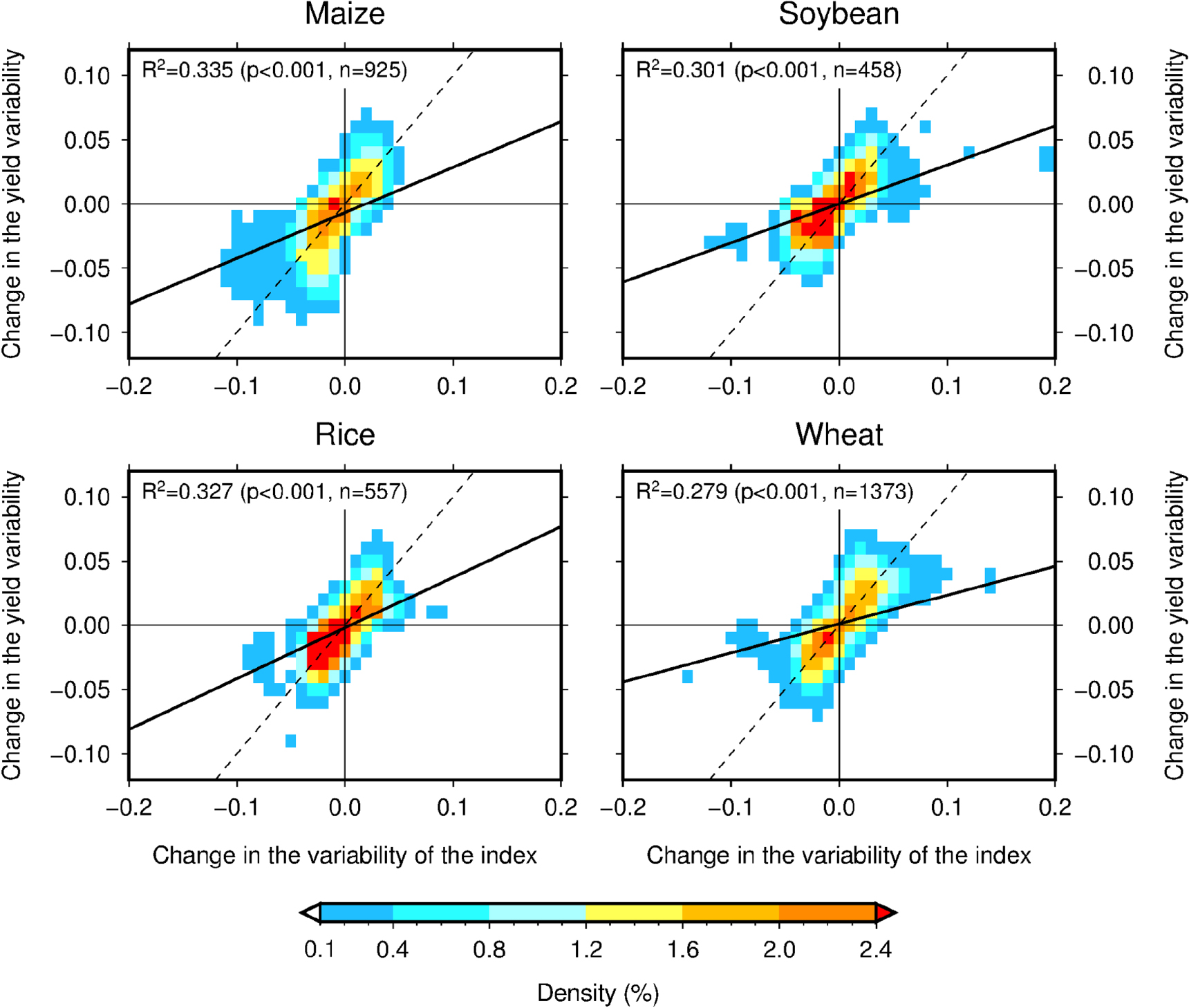
Standard image High-resolution imageThe geographic pattern of change in variability of the agro-climatic index was similar to that of yield variability change (figures S1 versus S5 and figures S2 versus S6). In the areas where the index was reliable (figure 3), 28%–34% of the yield variability change could be explained by change in the variability of agro-climatic condition when assessed using the RM–Slp method (p < 0.001, two-tailed test, figure 4). Other methods (figure S7) and other yield data type (figure S8) yielded similar results. The relationship shown here is not necessarily causal, but at least proposes a useful working hypothesis for future studies that, in a considerable portion of the global harvested area, change in growing-season climate variability accompanied yield variability change.

Figure 4. Smoothed density scatter plots of (x-axis) the grid-cell change in the variability of agro-climatic index indicated by the ensemble median of the index against (y-axis) grid-cell yield variability change for four crops. Data derived from RM–Slp method and hybrid yield estimates are presented. Only the data at the locations where the index could reliably explain the major characteristics of yield variability change were used. The coefficient of determination (R2), p-value (p) and sample size (n) are presented. Dashed diagonal line indicates one-to-one line. Solid black line indicates the best-fit linear regression line.
Download figure:
Standard image High-resolution image3.3. Relative contribution of each abiotic stress to yield variability change
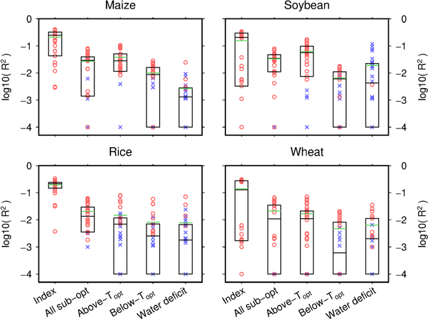
We next investigated which abiotic stress has most influenced yield variability change. As noted earlier, we computed the relative frequency of the three abiotic stresses (temperatures above and below the optimal range for yield formation and soil water deficit) as sub-indices using the same data as the index calculation and derived its variability change. The result derived from RM–Slp method suggests that the variability change of the relative frequency of suboptimal condition partly explains yield variability change (All sub-opt, figure S9; 2%–9% of the variance explained or about one-fourth of the 28%–34% change in variability of the index shown in figure 4). Temperature above the optimal range for yield formation (above-Topt) explained almost the same percentage of variance (2%–10%) (figure S9). For temperature below the optimal range for yield formation and soil water deficit during the yield formation stage, no significant relationship to yield variability change was found; or a significant relationship emerged but the explained variance was negligible (<3%, below-Topt and water deficit, figure S9). These tendencies consistently appeared across the crops with some uncertainties associated with different methods, yield data types and assumptions on local management and technology (figures 5 and S10). These findings provide empirical evidence that variability change of the relative frequency of suboptimal condition, especially temperature above the optimal range for yield formation, accompanied yield variability change. However, note that the influence of climate change on yield variability is complex—climate change till now has led to both decrease and increase in yield variability (figures 4, S7 and S8).
Figure 5. Comparison of the skill in explaining yield variability change across different sub-optimal conditions for four crops. The skill was indicated by the coefficient of determination (R2) calculated between the grid-cell yield variability change (derived using the hybrid yield estimates) and the grid-cell change in variability of each sub-optimal condition. The sub-optimal conditions include the temperature above and below the optimal range for yield formation (above-Topt and below-Topt, respectively), soil water deficit during the yield formation stage and all three sub-optimal conditions (all sub-opt). Data for the change in variability of the agro-climatic index are presented as the reference. Red circle and blue cross indicates significant and insignificant R2 value at the 5% level. A box indicates 50% probability interval. Black and green horizontal line within a box indicates median and mean value, respectively. Data for each box plot were derived from four different methods (RM–Slp, RM–SDr, FD–Slp and FD–SDr) and seven different members (thus, the sample size for a box was 28).
Download figure:
Standard image High-resolution image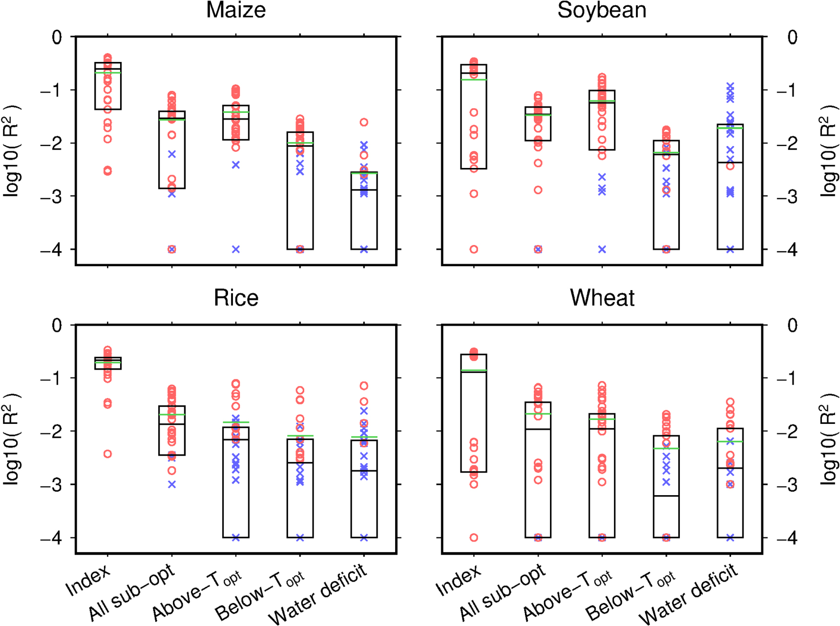
4. Discussion
4.1. Possible mechanisms leading to yield variability change
There were both decreases and increases in the variability of agro-climatic condition (figures 4, S7 and S8). These changes could be explained by the balance between seasonal and long-term changes in climate. Warming leads to more rapid crop growth and shifts the yield formation stage earlier (this often corresponds to cooler season before midsummer for the crops except winter wheat) [30–33]. This would decrease the number of days with temperature above the optimal range for yield formation during the yield formation stage, but at the same time both increase and decrease in the number of days with temperature below the optimal range for yield formation could happen depending on the amplitude of warming in cooler season and the degree of the acceleration of crop growth. If the increase in the number of days with temperature below the optimal range for yield formation was more prominent than the decrease in the number of days with temperature above the optimal range for yield formation then the variability of agro-climatic condition would increase, as previously suggested for warmer climate [30, 31]. In contrast, if the number of days with temperature below the optimal range for yield formation decreased and the number of days with temperature above the optimal range for yield formation also decreased, then agro-climatic index would become less variable.
Potential evapotranspiration rate during the cooler season is in general lower than that in the warmer season. However, change in the number of days with soil water deficit in the yield formation stage varied by location and crop because of many factors, such as precipitation seasonality, memory of soil moisture, the amplitude of long-term changes in temperature and precipitation and their interactions. For instance, our results show that the agro-climatic condition for maize and soybean in American Midwest became more stable than before (figures S5 and S6). This change is qualitatively consistent with the reported increase in summer precipitation and associated slowdown of increase in summer temperature in this region [34–36].
4.2. Implications
Our analysis revealed that yields of major crops in some regions of the world, including both major crop-producing regions and relatively food-insecure regions, have become more unstable, while yields in many more regions have become stable over time. Examples of major crop-producing regions with increased yield variability include maize and soybean in Argentina and Northeast China, rice in Indonesia and Southern China, and wheat in Australia, France and Ukraine. Maize in Kenya and Tanzania and rice in Bangladesh and Myanmar are the examples of relatively food-insecure regions with increased yield variability. Some of these changes, such as maize in China, rice in Bangladesh and wheat in Australia and France, have already been reported [21]. Also our finding that, at the global scale, rice yield variability decreased in many more regions than it increased, and the comparable area with decreased and increased wheat yield variability (figures 2, S1 and S2), are consistent with the previous results that the decrease in the variability of global-mean yield of rice is more prominent than that of wheat [21]. Unlike previous studies, we have been able to attribute a substantial portion of change in yield variability to climate change in a statistically significant manner. We believe the improved attribution is due to the use of spatially-explicit yield data, daily weather data, and agro-climatic index approach based on relatively process-based understanding, compared to previous studies that used national yield data, monthly climate data and simple regression models.
For other location–crop combinations, our results are qualitatively comparable to previous results although only a limited number of comparisons are available because most studies analyzing a climate-yield relationship examined year-to-year yield variability, but not trends in yield variability. For instance, the decreased maize yield variability in the Unites States (figures 2, S1 and S2) is consistent with the result presented in [18], although only the period 1981–2000 overlapped between the two studies. Our results of decreased maize yield variability in major-producing area in France and increased yield variability in minor-growing area matches with the overall decrease in maize yield variability at a national level reported by [19].
Our findings show that a decrease in yield variability is a major trend worldwide across the crops examined here. On the other hand, crop yields in some regions of the world have become more unstable. These results suggest the need for long-term global yield monitoring such as the ongoing international initiative on global crop monitoring [37]. At the moment of writing, increased yield variability does not seem to be a strong trend to call for an urgent response of many national governments, but is important for some regional economies. If the trend toward an increase in yield variability lasts and becomes more widespread, then it should have larger implications for national governments and commercial entities in food-importing countries as well as international food and humanitarian agencies to transform their food supply systems to be more robust. However, note that this view is only based on the mean trend in yield variability in the recent past. Changing climate extremes associated with changes in mean climate and associated severe yield losses could rapidly alter the trend. The finding of this study thus does not decrease the importance of ongoing adaptation efforts.
4.3. Limitations
This study has some limitations. A single index was associated with yield variability. While some sub-indices were used to infer potential mechanisms, these are not independent of the main index. The addition of indicators related to extreme excess soil water or floods into the analysis may be desirable. Furthermore, historical information on technology is lacking. The fact that we only used the time-constant technological data may explain the relatively limited skill of the index in explaining yield variability change because some studies have reported the importance of technological change modifying the yield response to climate [18–20, 38]. Particularly, the expansion of irrigated area is a well-known reason for decreased regional yield variability [18, 19]. A global historical data set of technology does not yet exist ([39] is a notable exception although it does not provide crop-specific information), but may be available for a limited region. Crop genetics may be another reason. Other limitations related to the models used to derive the index are discussed in section S2.5.
5. Conclusions
This study presented a spatially-explicit global analysis detecting yield variability change in the recent past and attributing it to climate change. Our analysis revealed that variability change in the relative frequency of temperatures exceeding the optimal range for yield formation has accompanied yield variability change in many crop-location combinations. Both decrease and increase in yield variability have been driven by climate change till now depending on the crop and location, suggesting the importance of long-term global yield monitoring and data collection to understand the ongoing yield variability change and its drivers.
Attributing changes in yield variability using historical data and more sophisticated process-based models [35, 40, 41] are encouraged for better understanding of the separate contributions of climate, technology, management and policy. Understanding the relationship between yield variability change and yield stagnation [15, 42] is a potential way forward to develop synergic adaptation technologies that could decrease yield gap while stabilizing yield variability.
Acknowledgments
TI thanks G Sakurai for sharing the computational code for Bayesian calibration and M Yokozawa, M Nishimori, D Makowski, T Ben-Ali and AJ Challinor for their comments at earlier versions of this study. TI was partly supported by the Environment Research and Technology Development Funds (S-10 and S-14) of the Ministry of the Environment, Japan and by JSPS KAKENHI Grant Number: 26310305. NR was supported by a Discovery Grant from the Natural Science and Engineering Research Council of Canada (NSERC).