

Abstract
The zero emissions commitment (ZEC) is the expected temperature change following the cessation of anthropogenic emissions of climate altering gases and aerosols. Recent model intercomparison work has suggested that global average ZEC for CO2 is close to zero. However there has thus far been no effort to explore how temperature is expected to change at spatial scales smaller than the global average. Here we analyze the output of nine full complexity Earth System Models which carried out standardized ZEC experiments to quantify the ZEC from CO2. The models suggest that substantial temperature change following cessation of emissions of CO2 can be expected at large and regional spatial scales. Large scale patterns of change closely follow long established patterns seen during modern climate change, with higher variability and more change as one approaches the polar regions, and with more change over land than ocean. The sign of temperature change (warming or cooling) varies by model and climatic zone. At the regional scale patterns of change are far more complex and show little consistency between different models. Analysis of model output suggest that for most models these changes far exceed pre-industrial internal variability, suggesting either higher climate variability, continuing changes to climate dynamics or both. Overall substantial regional changes in climate are expected following cessation of CO2 emissions but the pattern, magnitude and sign of these changes remains highly uncertain.
Export citation and abstract BibTeX RIS

Original content from this work may be used under the terms of the Creative Commons Attribution 4.0 license. Any further distribution of this work must maintain attribution to the author(s) and the title of the work, journal citation and DOI.
1. Introduction
A key question for devising climate policy is: how much climate change are we committed to? To help answer this question a number of metrics have been devised to quantify committed climate change. These metrics include: 'constant composition commitment' which quantifies climate change following stabilization of greenhouse gas concentrations [1]; 'emission commitment' which quantifies future emissions from existing fossil fuel infrastructure [2]; and 'zero emissions commitment' (ZEC) the amount of climate change expected following the cessation of anthropogenic emissions of climate altering substances [3, 4]. While constant composition commitment has fallen out of use as the metric is easily misinterpreted to imply considerable committed warming [5], the other two metrics have respectively become important foci of the social science (e.g [6]) and natural science (e.g. [7]) aspects of the climate sciences.
ZEC can be conceptualized as the climate impact of ceasing all anthropogenic emissions [3], individual forcing agents [8], or only CO2 emissions [4]. Due to the relatively short life-time of forcing agents other than CO2 over decadal periods, with the notable exception of N2O, ZEC from all forcing agents tends to converge on CO2-only ZEC [8, 9]. Hence CO2-only ZEC has been the main focus of recent simulations of ZEC [7, 10]. The Zero Emission Commitment Model Intercomparison Project (ZECMIP) used the CO2-only conceptualization of ZEC, and constitutes the most recent deep exploration of the metric. Eighteen earth system models (ESMs), nine of full complexity and nine of intermediate complexity, participated in ZECMIP [7]. For the high priority ZECMIP experiment models follow the standard idealized 1pctCO2 experiment [11] wherein CO2 concentration rises at 1% per year compounded until each model diagnoses that 1000 PgC of CO2 has been emitted to the atmosphere, at which point they branch off to a zero-emissions experiment (esm-1pct-brch-1000PgC). Thereafter CO2 emissions are set to zero and atmospheric CO2 is allowed to evolve freely [10]. ZECMIP found that 50 years after emission cease, ZEC ranged from −0.36 to 0.29 ∘C, with a multi-model mean of  C. Thus MacDougall et al [7] concluded that at the global level ZEC is likely to be close to zero in the decades following cessation of emissions.
The magnitude of climate change is most commonly summarized with the global average change in near-surface temperature [12], and consequently the Paris Agreement to mitigate climate change is framed with the goal of staying well below 2 ∘C of global average warming [13]. Thus it was natural for the early work on ZEC to focus on the expected evolution of global average temperatures. However, few locations are expected to experience the same change in temperature as the global mean value, with large deviations from the global average at smaller scales being the norm in the historical record [14, 15]. Therefore there is a keen interest to examine ZEC on spatially resolved scales to determine how these smaller scale climates are expected to evolve after emissions cease.
The Intergovernmental Panel on Climate Change breaks the spatial scale of climate in large, regional, and local scales [14]. Large scale climate typically encompasses the scale of tropical, extra-tropical and polar climate zones, as well as oceans and continents, while regional climates encompass systems on the scale of subcontinental regions (e.g. the Caribbean) down to individual cities [14]. Local scale climates are at the scale of neighbourhoods, fields, and smaller, and are well below the resolution of climate model simulations [14]. In general for large scale climates the land and the Arctic have warmed faster than the global average but with higher inter-annual variability than oceans or the tropical regions [15]. Regional scale climates vary substantially due to complex interactions of local topography, ocean currents, feedback mechanisms and long-range tele-connections [14]. Here we will use the output from the full complexity ESMs that participated in ZECMIP to analyze ZEC at the large and regional scales.
2. Methods
2.1. Models
Here we examine the full complexity ESMs that participated in ZECMIP and have submitted their results to Earth System Grid Federation. Nine ESMs have done so: ACCESS-ESM1-5 [16, 17], CanESM5 [18], CESM2 [19, 20], GFDL-ESM4 [21], GISS-E-2.1 [22], MIROC-ES2L [23], MPI-ESM1-2-LR [24, 25], NorESM2-LM [26], and UKESM1-0-LL [27]. Notably this list of nine ESMs is different from the nine that were analyzed by MacDougall et al [7] in the initial ZECMIP analysis paper. In the initial analysis output from GFDL-ESM2M was analyzed, while for the submission to Earth System Grid Federation these simulations were replaced with the new version of the model—GFDL-ESM4. An additional model, GISS-E2.1, completed the ZECMIP experiments too late to be analyzed by MacDougall et al [7]. Additionally, as of August 2022, the ZECMIP results from CNRM-ESM2 have yet to be submitted to Earth System Grid Federation.
Succinct model descriptions for aspects of the model relevant for understanding ZEC for the seven models examined here and in MacDougall et al [7] are detailed in the appendices MacDougall et al [7]. A full description of the GFDL-ESM4 model is given by Dunne et al [21] and of GISS-E2.1 in Kelley et al [22]. Because the biogeochemical components of ESM are computationally expensive, many ESMs use lower resolution variants of their ocean and atmosphere components. Thus MIROC-ES2L, MPI-ESM1-2-LR, NorESM2-LM, and UKESM1-0-LL all use lower resolution versions of their atmosphere and ocean components than the general circulation variants of these models (See appendices of [7]). Notably lower resolution model variants are expected to have somewhat different patterns of warming relative to high resolution versions of the same model (e.g. [28]).
2.2. Model experiment
The ZECMIP protocol [10] outlined six experiments to quantify ZEC and its dependence on total emissions of CO2 and CO2 emissions pathway. Only one of these experiments, esm-1pct-brch-1000PgC, was requested from all participating full complexity ESMs. The esm-1pct-brch-1000PgC experiment branches from either the standard 1pctCO2 experiment [11] after models diagnose that 1000 PgC has been emitted to the atmosphere from burning of fossil fuels, or from the esm-1pctCO2 which is emission driven from the start of the simulation [10]. Neither the 1pctCO2 nor the esc-1pctCO2 experiments simulate land-use-change. Thereafter the models switch from concentration driven to emissions driven configurations and CO2 emissions are set to zero. Thus the atmospheric CO2 pool is allowed to freely evolve in response to changes in oceanic and terrestrial carbon pools [10]. Although this experiment is highly idealized [29] the instantaneous cessation of emissions allows for clear distinction between ZEC and the transient climate response to cumulative CO2 emissions [7, 30]. ESMs were requested to submit simulations of at least 100 years following cessation of emissions. While multiple ensemble members were not requested, two models—CESM2 and UKESM1-0-LL, did each submit three ensemble members to Earth System Grid Federation.
2.3. Analysis
To quantify ZEC at large spatial scales 2 m air temperature anomalies following cessation of emissions were computed for the land and oceans, as well as zonal averages for tropical, extratropical, and polar regions. For all computations the protocol devised for computing the global value of ZEC was followed [7]. That is, ZEC is taken as relative to the 20 year mean temperature from the 1pctCO2 experiment centred about the point in time where the esm-1pct-brch-1000PgC branches from the 1pctCO2 experiment [7]. Due to the sudden halt in the rate of temperature change in the esm-1pct-brch-1000PgC experiment, using the 1pctCO2 experiment in place of the esm-1pct-brch-1000PgC experiment is necessary to avoid an underestimation of the global temperature at the time of emission cessation [7]. The land-ocean mask provided for each model is used to separate land and ocean 2 m air temperatures and compute areally weighted mean values. For zonal averages Earth is divided into a tropical region extending from 30 ∘S to 30 ∘N, two extratropical regions one in each hemisphere between 30 ∘ to 60 ∘, the Arctic region above 60 ∘N, and an Antarctic region below 60 ∘S. Note that we have used divisions approximating the extent of the Hadley, Farrell, and Polar atmospheric circulation cells [31], instead of the astronomical definitions of these regions.
For regional climate our principal aim is to compute ZEC at the grid-point scale and investigate whether the patterns observed are due to internal variability or are being generated by persistent dynamically driven changes to regional climate. Following MacDougall et al [7] our main focus is on 50 years after emissions cease, a metric called ZEC50. To derive maps of ZEC50 we take a 20 year average for each grid-point centred at 50 years after emissions cease, and find the difference between these grid-point averages and the 20 year mean grid-point temperature from the 1pctCO2 experiment centred around the year emissions cease. To explore whether the resultant patterns are distinguishable from internal variability we use the following statistical metric:
where, A is a climate anomaly expressed as units of standard deviations (formally dimensionless), ZL is the local ZEC, and ZG is the globally averaged ZEC value of the respective model. σL is the local standard deviation of differences between pairs of 20 year average temperature anomalies. That is, σL quantifies how much variance one would expect between any two (non-overlapping) 20 year average temperatures at a given location. σL was calculated from the pre-industrial control simulation (pi-control) for each model. The control simulations were first detrended at each grid-point and then discreetly averaged into non-overlapping 20 year mean temperatures. Thereafter differences were found between every combination of 20 year mean temperatures at that grid-cell location and the standard deviation taken of these differences to compute σL . Providing a minimum 500 year pre-industrial control simulation (pi-control) wherein models are evolving under constant pre-industrial forcing was a requirement for entry into CMIP6 [11], and thus such a simulation exists for all models that participated in ZECMIP. Note that we have used that standard pi-control simulation where CO2 concentration is held constant. Evaluated over the whole planetary surface the metric can give a sense for whether a dynamic shift has taken place or that internal variability has increased relative to pre-industrial times. Generally the higher fraction of the surface exhibiting large absolute values of the metric indicates that it is more likely that such a shift has occurred. For example assuming a Gaussian (normal) distribution we would expect that 5% of the surface would have absolute values over 2, if we instead find that 25% of the surface has absolute values above 2 then it is likely that either dynamic changes have occurred or the internal variability has increased relative to pre-industrial times. The metric is a slight variant of the commonly used Standardized Mean Difference statistical metric. For conciseness we call this metric 'Regional Standard Difference'. The metric can be computed for any given time after emissions cease.
A more conventional way of removing internal variability and establishing the robustness of dynamic changes in ESM output is to average together many ensemble members from the same model conducting the same numerical experiment (e.g. [32]). However only two of the models submitted more than one ensemble member, and these models submitted only three members each. Sample sizes of three are not kind to the reliability of formalized statistical metrics, however the range of values between these ensemble members is nonetheless informative about the persistence of dynamic changes.
3. Results
3.1. Land and ocean ZEC
Figure 1 shows ZEC for the land and ocean area for each model. In general the response over land is more extreme and more variable than over the ocean. Over land three of the models (CESM2, MPI-ESM1-2, and MIROC-ES2L) have cooled by more than 0.5 ∘C by the end of their simulations, after 150 years, while over the ocean no model breaches that cooling threshold. Other models such as ACCESS-ESM1-5 and GISS-E2.1, show a more moderate response with both land and ocean ZEC staying close to zero. One model (UKESM1-0-LL) shows substantial warming of similar magnitude over both the land and the ocean, although with much higher variability over land. The ZEC50 values for land and ocean are shown in table 1. Seven of the models have negative ZEC50 over the land and the ocean, with ZEC50 over the land being on average 0.15 ∘C cooler than over the ocean. Note that due to a slightly different collection of ESMs than that assessed in MacDougall et al [7] the multi-model, global mean value of ZEC is lower than that previously assessed. As this is largely due to one of the higher ZEC models being slow to upload their data to Earth System Grid Federation this should not be interpreted as a meaningful change.
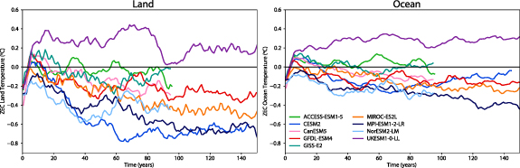
Figure 1. ZEC over land (left) and over the ocean (right). ZEC is the temperature difference from the global temperature at the time when emissions cease. An 11 year moving average has been applied to smooth the model output. Yearly averaged temperatures are shown in the supplementary information (figure S1). The moving average creates the artifact whereby lines begin below zero.
Download figure:
Standard image High-resolution imageTable 1. ZEC 50 years after emissions cease (ZEC50) for land, ocean, and globally.
| Model | Land ZEC50 (∘C) | Ocean ZEC50 (∘C) | Global ZEC50 (∘C) |
|---|---|---|---|
| ACCESS-ESM1-5 | −0.06 | 0.04 | 0.01 |
| CESM2 | −0.61 | −0.18 | −0.31 |
| CanESM5 | −0.17 | −0.07 | −0.14 |
| GFDL-ESM4 | −0.26 | −0.18 | −0.21 |
| GISS-E2.1 | −0.15 | −0.03 | −0.06 |
| MIROC-ES2L | −0.21 | −0.06 | −0.08 |
| MPI-ESM1-2-LR | −0.37 | −0.23 | −0.27 |
| NorESM2-LM | −0.51 | −0.26 | −0.33 |
| UKESM1-0-LL | 0.28 | 0.29 | 0.28 |
| Mean | −0.23 | −0.08 | −0.12 |
| Median | −0.21 | −0.07 | −0.14 |
| Standard deviation | 0.26 | 0.17 | 0.19 |
Simulations with general circulation models long ago established that land areas are expected to warm more than the ocean even when the climate system has come into full equilibrium with a change in radiative forcing [33]. This persistence anomaly was diagnosed to be caused by inter-linked changes in humidity, lapse-rate and moisture transport affecting local radiative transfer in the atmosphere over the continents [33]. How these processes will interact with changes in ocean heat uptake in a scenario of zero emissions is unclear and likely a fruitful avenue for further research.
3.2. Zonal averages
Figure 2 show the zonal averages for ZEC for each model. The figure shows clear zonal differences in ZEC, with ZEC being closer to zero, less variable, and exhibiting smaller trends in the tropical region compared to other regions (recall that the tropics cover half the planetary surface). The southern hemisphere mid-latitudes show remarkably little inter-annual variability and ZEC values close to zero, however, continuing warming trends in CESM2 and UKESM1-0-LL are clear. Note, that the southern hemisphere mid-latitudes are dominated by the Southern Ocean, and contain very little land. The northern hemisphere mid-latitudes are more variable and are generally consistent with ZEC over land (figure 1(a)), which is unsurprising given the extent of continents in this region. Both Arctic and Antarctic exhibit high variability, both in time and between models, with more variability in the Arctic relative to the Antarctic. It is noteworthy that the three models experiencing strong negative ZECs over land after 150 years, are the ones showing the strongest cooling over the Arctic region.
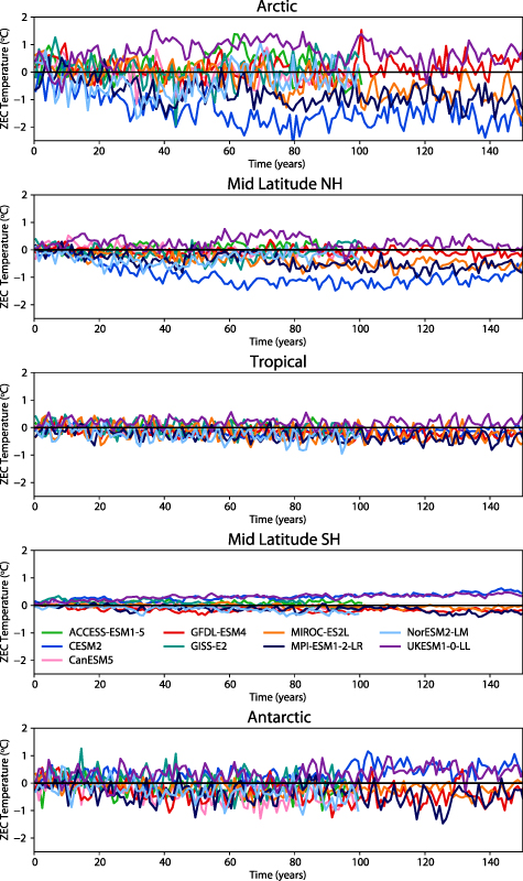
Figure 2. ZEC for zonal climate regions. The tropical region extends from 30 ∘S to 30 ∘N, extratropical regions between 30 ∘ and 60 ∘ in each hemisphere, the Arctic region above 60 ∘N, and an Antarctic region below 60 ∘S.
Download figure:
Standard image High-resolution imageTable 2 shows the ZEC50 values for the zonal regions. The changes in the Arctic are most striking with some models showing a ZEC close to zero (MIROC-ES2L and CanESM5), others showing almost 1 ∘C of warming (UKESM1-0-LL), and another over 1 ∘C of cooling (CESM2). The bounds of Arctic ZEC extend between  C and 2 ∘C (figure 2). The tropics in contrast exhibit a range of ZEC50 from −0.31 to
  C. Five of the nine models agree in the sign of change in ZEC50 for all zonal regions (CanESM5, GFDL-ESM4, MPI-ESM1-2-LR, NorESM2-LM, and UKESM1-0-LL), while the other four show broad zonal regions of warming and cooling.
Table 2. ZEC 50 years after emissions cease (ZEC50) for zonal climate regions. NH is Northern Hemisphere, SH is Southern Hemisphere.
| Model | Arctic ZEC50 (∘C) | NH mid-latitude ZEC50 (∘C) | Tropical ZEC50 (∘C) | SH mid-latitude ZEC50 (∘C) | Antarctic ZEC50 (∘C) |
|---|---|---|---|---|---|
| ACCESS-ESM1-5 | 0.29 | 0.02 | −0.02 | 0.07 | −0.21 |
| CESM2 | −1.36 | −0.98 | −0.20 | 0.25 | 0.21 |
| CanESM5 | −0.10 | −0.16 | −0.05 | −0.03 | −0.53 |
| GFDL-ESM4 | −0.09 | −0.12 | −0.21 | −0.22 | −0.49 |
| GISS-E2.1 | −0.18 | −0.32 | 0.00 | 0.05 | 0.02 |
| MIROC-ES2L | 0.05 | −0.34 | −0.08 | 0.01 | −0.17 |
| MPI-ESM1-2-LR | −0.76 | −0.28 | −0.25 | −0.10 | −0.35 |
| NorESM2-LM | −0.68 | −0.48 | −0.31 | −0.11 | −0.38 |
| UKESM1-0-LL | 0.94 | 0.23 | 0.21 | 0.32 | 0.34 |
| Mean | −0.21 | −0.27 | −0.10 | 0.03 | −0.17 |
| Median | −0.10 | −0.28 | −0.08 | 0.01 | −0.21 |
| Standard deviation | 0.66 | 0.34 | 0.16 | 0.17 | 0.31 |
3.3. Regional climate
Maps of ZEC50 for each ESM are shown in figure 3. The patterns suggest that many regions can expect substantial climate change following cessation of emissions. At the extremes, UKESM1-0-LL has a grid-cell with a ZEC of 5.10 ∘C and GISS-E2.1 has a grid-cell with a ZEC50 of  C. Each ESM exhibits a unique pattern of regional warming and cooling with few consistent features between models. These range from relatively uniform cooling in NorESM2 to patchy warming and cooling in a number of models, to the strong inter-hemispheric gradient in CESM2. General patterns that can be spotted are a stronger cooling over land compared to the ocean, as well as a high ZEC response in the Arctic region, confirming the signals found in the zonal means of section 3.1.

Figure 3. Maps of ZEC 50 years after emissions cease (ZEC50) for each ESM.
Download figure:
Standard image High-resolution imageFigure 4 shows changes in temperature 50 years after emissions cease relative to the change in temperature at the time emissions cease. The figures show how climate change after emissions cease compares to the climate change already experienced before emissions cease. These relative changes show somewhat more consistent patterns with all of the models showing anomalies of various sizes and magnitudes in the North Atlantic, with these anomalies being most extensive in CESM2 and GISS-E2.1. The other region where large relative changes occur in all models after cessation of emissions is the Southern Ocean, with an expanse in the South Pacific being a particularly anomalous region in most models. Overall very little of the planetary surface is expected to return to pre-industrial temperatures (median 1.7%, range of 0.1%–3.78% of the planetary surface cooling to pre-industrial temperature), and likewise only a small fraction of the planetary surface is expected to warm more in the 50 years after emission cease than warmed by time emission ceased (median 0.5%, range of 0%–1.9% of the planetary surface warming more in the 50 years after emissions cease than before).

Figure 4. Maps of ZEC50 values relative to the change in temperature when emissions ceased. A value of −100% indicated that the climate has returned to pre-industrial temperatures, while a value of 100% indicated that the location has changed temperature as much after emissions cease as it did before emissions ceased. Note that some models project a region in the North Atlantic that has cooled relative to the pre-industrial climate by the time emissions cease, creating the rapid transition between values of −100% to 100% as the warming to cooling boundary is crossed. Simulations branch from the 1pctCO2 experiment 61 to 70 years after the beginning of the 1pctCO2 experiment.
Download figure:
Standard image High-resolution imageThe diverse patterns seen in the spatially resolved ZEC50 in the model output leads to the question of whether the patterns that are seen are persistent or are being driven by internal variability. The best way to answer such a question would be to examine a large ensemble of simulations from each model conducting the experiment. However, only a small ensemble (three members each) is available for two of the models. Figure 5 shows the ensemble mean and range for CanESM5 and UKESM1-0-LL. Both ensemble means show persistent patterns between the three ensemble members. CanESM5 exhibits warming in the North Atlantic and cooling in the Southern Ocean and UKESM1-0-LL exhibits strong Arctic warming. The range between the ensemble members shows that both models exhibit more internal variability over the Arctic, Antarctic, and Southern Ocean, and smaller and consistent variability between 45 ∘ North and 30 ∘ South. These results suggest that the patterns observed in figure 3 are created by a mix of internal variability and persistent dynamically driven changes in regional climate.
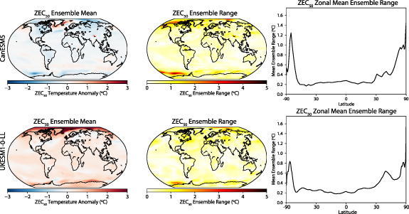
Figure 5. Ensemble mean (left column), ensemble range (middle column), and zonal mean of model range (right column), for the two models which conducted multiple ensemble simulations of the ZEC esm-1pct-brch-1000PgC experiment. Note that the X-axis for zonal mean of model range is weighted to the fraction of the planetary surface area in each zonal band.
Download figure:
Standard image High-resolution imageFigure 6 shows maps of the Regional Standard Difference (see section 2.3) for each of the models. Two of the models, ACCESS ESM1-5 and GFDL-ESM4, show values within the −2 to 2 standard deviation range that would be expected for Gaussian (normal) distributions. The other ESMs show extensive regions outside this range, particularly in the Southern Ocean and North Atlantic. In addition, UKESM1-0-LL has values far outside the −2 to 2 standard deviation range in the Arctic, and CESM2 has extensive regions outside this range of opposite signs in both hemispheres. Figure 7 shows the fraction of the planetary surface above a given absolute value of regional standard difference for each model, along with a reference value for a Gaussian distribution of the same metric. Figure 7(a) shows this for an example from the pre-industrial climate and figure 7(b) for 50 years after emissions cease. For the pre-industrial climate values are close to the Gaussian expectation, with some models above and some below this line. For the ZEC50 climate all models are either equal to or above the Gaussian expectation. This indicates that for most models the ZEC climate is exhibiting either an increase in variability relative to the pre-industrial climate, large dynamically driven changes in regional climate, or a combination of both.
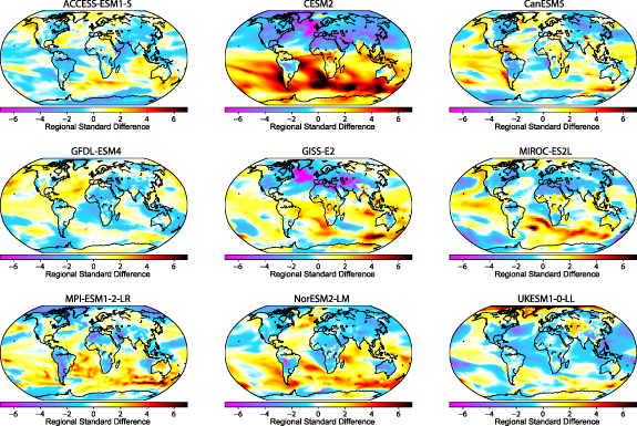
Figure 6. Maps of Regional Standard Difference 50 years after emissions cease (see section 2.3. Units are standard deviations (dimensionless).
Download figure:
Standard image High-resolution image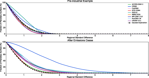
Figure 7. Fraction of the planetary surface above a given absolute value of Regional Standard Difference measured in standard deviations. The pre-industrial example is simply the last 20 year block of time from the de-trended pre-industrial control simulation relative to the first 20 year block of time. Note that ESMs are complex deterministically chaotic systems and not truly stochastic [34].
Download figure:
Standard image High-resolution image4. Discussion
The analyses have shown that across different ESMs large regional differences for ZEC50 exist. Overall, inter-model variance in ZEC over land is higher than over the ocean, however, the Arctic region (north of 60 ∘N) is the region experiencing the highest inter-model variance and interannual variability within models (figures 1 and 2). The zonally resolved ZEC50 analyses show that in addition to the Arctic Ocean, the North Atlantic and the Southern Ocean are especially sensitive to changes in temperature 50 years after cessation of emissions (figures 3 and 4). Overall, our analysis suggest that models exhibiting an increase in variability relative to the pre-industrial climate, large changes in regional climate dynamics or possibly both (figures 6 and 7). In the following we will outline three possible interlinking mechanisms creating these signals to provide a direction for further research into the dynamic drives of post-emissions climate change.
Firstly, the difference in the order of magnitude of warming between the land and ocean temperature signals after emissions cease, is likely explained by the different heat capacities of these two bodies. Generally, land temperatures are quicker to reverse toward their pre-industrial temperatures, which is the reversed trend currently observable under climate change, where land surface heats up faster than the ocean (e.g [14]). That is, land is expected to continue to warm and cool faster than the ocean, a climate pattern consistent with very well established phenomena such as day-night temperature range, seasonal temperature range, and historical global warming [15].
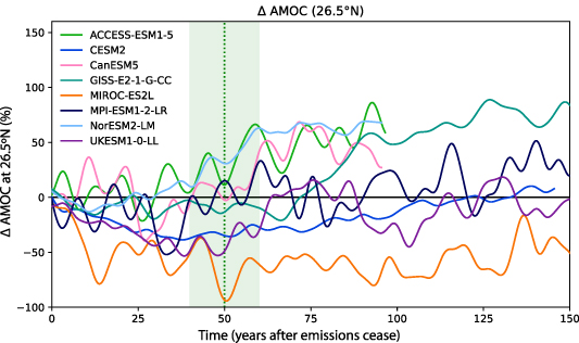
Our second proposed mechanism is the evolution of Atlantic Meridional Overturning Circulation (AMOC) following cessation of emissions. A hypothesis born from the anomalies of various magnitudes seen in the North Atlantic region, the region with a dominant wind-driven part of the AMOC, (figure 6) as well as results of previous studies that have examined AMOC evolution during simulated periods of net-negative emissions [35, 36]. To explore this hypothesis the strength of AMOC (at the Rapid Observational Array latitude of 26.5 ∘N [37]) is show in figure 8. Fifty years after emissions cease AMOC recovery varies strongly between the models. While some already show signs of AMOC strengthening (NorESM2-LM, ACCESS-ESM1-5), some show continuous decline after 50 years (CESM1, UKESM1-0-LL, MIROC-ES2L). The signal of reduced northward heat flux is suggested by the ZEC50 temperature maps, as a cooling signal in the North Atlantic Ocean along the Gulf Stream and North Atlantic current (between 40 ∘ and 50 ∘N) (see figure 3). Inter-model differences in the impact to AMOC recovery are sensitive to latent heat flux, specific humidity and low cloud dynamics within the models [35], and will have to be subject for further study.
Figure 8. Change in Maximum AMOC strength (AMOC) excluding the top 500 m at 26.5 ∘N normalized to the decrease in AMOC between preindustrial and cessation time with respect to the value at cessation. Smoothing has been applied.
Download figure:
Standard image High-resolution image
A third mechanism which may be contributing to the large-scale and regional patterns of ZEC50 are changes in sea-ice extent and, the associated strength of the ice-albedo feedback. To explore the viability of this mechanism figures S2, and S3 show changes in sea-ice extend in September and February respectively. The figures show a coincidence between recovery of ice area and cooling during zero emissions, hinting at a high sensitivity of regional ZEC50 temperature response to the ice albedo feedback within models. These signals can also be seen in the ensemble range of CanESM5 and UKESM1-0-LL, showing high ranges in the Arctic Ocean and in front of the West Antarctic peninsula, in the Pacific part of the Southern Ocean (figure 5). Inter-model differences in the strength of the ice-albedo feedback during this period of possible sea-ice recovery point to the importance of the representation of atmospheric properties like the Arctic cloud effect within models [38].
In addition to the three mechanisms outlined above other processes are likely contributing to regional patterns of ZEC. Two potential mechanisms that deserver further scrutiny are the effect of changes in cloud climatology on regional ZEC [39, 40], and the local scale radiative forcing effects that have been shown to contribute to land-sea warming contrast [33]. ZEC simulations have varying CO2 concentration between models as CO2 freely evolves in these experiments [7], which may contribute to radiative forcing derived differences between models.
One of the complexities we have outlined in our analysis of ZEC at regional scales is separating enhanced internal variability from persistent dynamic changes to climate. The best way to assess both effects is to analyze a large ensemble of simulations of the same experiment with the same model. Thus we recommend that the ZECMIP-II protocol request ESMs provide 10 ensemble members for 100 years for the top-tier simulation.
Climate change at regional and local scales is the climate change which has the greatest affect on human life and wellbeing [14]. The fact, that regional and thus likely local climates are expected to continue to substantially change following cessation of CO2 emissions is disconcerting. Gaining a better understanding of the likely sign and magnitude of these changes will be crucial for planning climate mitigation and adaptation efforts in the future. Given the large inter-model differences in the patterns of changes, focused efforts are needed to better understand the underlying processes driving these changes.
5. Conclusion
We have explored how temperature is expected to evolve following the cessation of CO2 at large and regional scales. At large scales there is strong model consensus that the patterns of temperature change will follow long-established precedents, with more change over land than the ocean, and with higher variability and a larger magnitude of change the further away from the tropics a location is. At regional scales the evolution of temperature is far more complex and there is little consensus between models, although some patterns do become evident when examining higher order statistics. Some models show relatively uniform changes at a given latitude with regional anomalies consistent with internal variability, while at the other extreme one model shows a large inter-hemispheric gradient in temperature change with warming in the southern hemisphere and cooling in the northern hemisphere. Examination of the small number of ensemble simulations available suggests that dynamic changes to climate are occurring in some models, while examination of patterns of temperature change relative to pre-industrial variability suggest that most models simulate either a increase in climate variability, dynamic changes to climate or a combination of both.
Analysis shows that both AMOC and sea-ice area evolve substantially in many models following cessation of emissions. Both of these processes are know to strongly affect regional climate [35, 38], and regional anomalies in ZEC50 are concentrated in the North Atlantic and sub-polar regions most affected by these two processes. However, focused research is needed to firmly establish causal relationships for the large regional temperature trends seen in most simulations. Overall we assess that it is likely that regional climate will continue to evolve substantially following cessation of CO2 emissions, despite global temperature change being close to zero.
Acknowledgments
A H M D is thankful for support from the Natural Sciences and Engineering Research Council of Canada (NSERC) Discovery grant program and for support from Compute Canada. J M is grateful for support from the NSERC Undergraduate Students Research Award program. N M and D H are funded under the Emmy Noether scheme by the German Research Foundation FOOTPRINTS—From carbOn remOval To achieving the PaRIs agreemeNts goal: Temperature Stabilisation (ME 5746/1-1).
Data availability statement
The data that support the findings of this study are openly available at the following URL/DOI: https://esgf.llnl.gov/.
Supplementary data (15 MB PDF)