

Abstract
A transient two-dimensional acoustic boundary element solver is coupled to a potential flow boundary element solver via Powell's acoustic analogy to determine the acoustic emission of isolated hydrofoils performing biologically-inspired motions. The flow-acoustic boundary element framework is validated against experimental and asymptotic solutions for the noise produced by canonical vortex-body interactions. The numerical framework then characterizes the noise production of an oscillating foil, which is a simple representation of a fish caudal fin. A rigid NACA 0012 hydrofoil is subjected to combined heaving and pitching motions for Strouhal numbers ( ) based on peak-to-peak amplitudes and chord-based reduced frequencies (
 ) that span the parameter space of many swimming fish species. A dipolar acoustic directivity is found for all motions, frequencies, and amplitudes considered, and the peak noise level increases with both the reduced frequency and the Strouhal number. A combined heaving and pitching motion produces less noise than either a purely pitching or purely heaving foil at a fixed reduced frequency and amplitude of motion. Correlations of the lift and power coefficients with the peak root-mean-square acoustic pressure levels are determined, which could be utilized to develop long-range, quiet swimmers.
Export citation and abstract BibTeX RIS

Original content from this work may be used under the terms of the Creative Commons Attribution 4.0 license. Any further distribution of this work must maintain attribution to the author(s) and the title of the work, journal citation and DOI.
1. Introduction
Many aquatic animals oscillate their fins to propel themselves quickly through the ocean. Their propulsion is based on an unsteady flow paradigm that is distinct from the steady flow paradigm that underpins the design of most man-made underwater vehicles. Consequently, animals can excel at maneuvering and rapid accelerations [1, 2] in addition to high-speed and high-efficiency swimming [3, 4]. This multi-modal performance has spurred vigorous research over the last two decades into bio-inspired autonomous underwater vehicles (BAUVs) [5–8], which would possess the additional benefit of exceptional stealth [9, 10]. It is generally expected that fish-like swimming motions lead to quiet acoustic signatures [9], which (even if detected) would resemble the noise signature of real fish, making a BAUV exceptionally difficult to detect and identify [11]. The quantification of noise signatures of swimming animals and BAUVs to date is minimal, and the trade-offs between noise generation and hydrodynamic performance of unsteady swimmers is necessary to assess such bio-inspired designs and devices for practical use. Further investigations into the competition between fluid dynamic performance and acoustic stealth could be beneficial in the realization of biologically-inspired aerial vehicles that aim to achieve novel flow-noise suppression [12–15].
Most sounds produced by fish result from aggressive actions, spawning, or reproductive behavior [16]. The noise made during these actions can be categorized into two broad categories: active acoustic signaling through morphological structures and passive noise generated during swimming, feeding, or respiration. The actively-produced noises include vocal calls, swimbladder motions, and drumming [17, 18]. Active fish signaling is not of interest here, as there exist quantified data for several species [17]. However, fish produce a vortex wake by simply oscillating their fins during swimming, which is a well-known source of noise [16]. Yet, the locomotive noise of fish during steady-state rectilinear swimming remains relatively unquantified. Fish locomotion produces low-amplitude hydrodynamic noise that is challenging to record reliably and has received limited attention in the literature [16].
Instead of examining live fish, numerical tools can be used to simulate the motions of fish and their resulting unsteady vortical wakes to estimate their noise production. For instance, one approach to simulating the unsteady flow field around a swimming fish is the boundary element method (BEM) [19]. This potential flow method discretizes surfaces representing shear layers in the flow, i.e. a solid body surface and the wake, into a collection of elements [20, 21]. This method approximates the flow as incompressible, inviscid, and irrotational (except on the elements). The unsteady flow phenomena is defined as a function of strengths of elements across the boundary, thereby reducing the domain and enabling rapid simulations. Far-field noise production of an airfoil in turbulent flow has been determined through a similar method by Glegg and Devenport [22]. A frequency-domain acoustic far-field was quantified by defining the forcing function of a BEM as the surface loading due to the energy spectrum of the turbulent boundary. However, this method is restricted to single airfoils in steady flows and does not account for interactions that would be present in many-bodied systems of swimmers or fliers. Computational fluid dynamics techniques such as fluid splitting methods can simulate the complete flow fields and therefore the unsteady and acoustic fields due to foil motions [23], but they are computationally expensive in comparison to the BEM. Once an unsteady flow field is simulated, an acoustic analogy is a common and effective tool to post-process the flow data and determine the noise production [24, 25]. The first acoustic analogy was developed by Lighthill [26] as a reformulation of the Navier–Stokes equations into a wave equation in terms of perturbations of the fluid density. The approach described by Lighthill has become nearly ubiquitous in flow noise and aeroacoustic studies [24, 25, 27, 28]. Adaptations to the Lighthill formulation have further simplified flow noise predictive systems, such as the recasting by Powell [29] of all unsteady flow fluctuations into vorticity and thereby making vorticity the forcing function of the system. Vorticity also plays a central role in the noise theory by Howe [30] that is adapted from Lighthill's formulation.
Motivated by these observations, the present study makes two principal technical advancements. First, a coupled flow-acoustic BEM is developed to predict the noise generation and performance of hydrofoils in unsteady motion that can also account for multi-body interactions, such as those that occur in fish schools. Second, the novel flow-acoustic BEM will be used to examine the performance and noise production of a hydrofoil in combined heaving and pitching motions, which acts as a simple, two-dimensional representation of an oscillating fish caudal fin. This paper is laid out across three main sections. The first section details a potential flow and acoustic BEM employed through the current study. Next, the coupling between the potential flow and acoustic solvers is presented along with validations of the solver against available experimental data and asymptotic solutions of vortex-body interaction noise. Finally, the performance and noise production of a combined heaving and pitching hydrofoil are examined with respect to non-dimensional frequency, amplitude, and heave-to-pitch ratio.
2. Materials and methods
2.1. Potential flow BEM
The following section provides a brief description of a two-dimensional unsteady potential flow BEM utilized for the present study. The method has been adapted from the work of Willis et al [31]. The flow solver, commonly called a panel method, solves the Laplace equation for a non-penetrable hydrofoil. The surface of the hydrofoil  is represented with a distribution of sources and doublets, doublets on an edge panel
  , and a collection of vortex particles in the wake
  (cf figure 1). The resulting distributions define a scalar potential that may be written as
where  is the outward unit normal of the surface, s is a source location, r is the observer location, and
  is the two-dimensional Green's function for the Laplace equation. The strengths of the source and doublet are defined respectively as
  and
and  where
where  is the potential of the interior of the body. The velocity induced by the vortex particles in the field
  , the body velocity U, and the velocity of the center of each element relative to the body-frame of reference
  are the parameters of the source distribution and ensure the no-penetration boundary condition.

Figure 1. Schematic of a fish with a blown up section depicting the propulsor as the discrete geometry for the BEM. A propulsor of chord length c is discretized with source/doublet elements (blue lines with endpoints indicated by black circles). The edge and buffer panels (green lines with endpoints indicated by green circles) are connected to the trailing edge of the propulsor. The vortex particle wake (blue/red circles) is shed from the edge/buffer panels.
Download figure:
Standard image High-resolution imageDiscrete, radially-symmetric, desingularized Gaussian vortex particles are used to define the domain vorticity. The evolution of vorticity in the domain is determined by the vorticity transport equation, which is simplified by the use of inviscid particles. The vortex blobs have an induced velocity determined by the Biot–Savart law [32],
where  is the circulation of the ith vortex particle, and
  is the cut-off radius. Following the work of Pan et al [33], the cut-off radius is set to
  for time step
  to ensure that the wake particle cores overlap and a thin vortex sheet is shed. The evolution of the vortex particle position is updated using a forward Euler scheme [31],

At each time-step, an implicit Kutta condition ensures that the vorticity at the trailing edge of the foil is zero. The iterative method employed is similar to the techniques described in [31, 34]. Vorticity is defined at the trailing-edge as doublets on two edge panels to satisfy the Kutta condition [31, 34]. The first edge panel directly follows from the trailing-edge, defining the circulation needed to satisfy the Kutta condition. Aft of the first edge panel is a virtual buffer panel that stores the time history of the first panels circulation before being released as a vortex particle into the wake. Figure 1 illustrates the distinction of the source/doublet panels across a foil, the arrangement of the trailing-edge and buffer panels, and how the vortex particle wake behaves behind the body.
The pressure calculation put forth by Katz and Plotkin [21] is augmented by the induced velocity of the vortex particle wake. The surface pressure is determined by
where  is the time rate of change due to a vortex particle with circulation Γ at an angle θ from the observation point. Equation (4) is similar to the form put forth by Willis et al [31], but here
  is the positional change of a vortex with respect to a panel and does not require the solution of a secondary system to find the influence of wake vortices onto the body surface. The appendix presents validation of this methodology against available theoretical and numerical results.
2.2. Acoustic BEM
The Helmholtz wave equation for a homogeneous medium and its boundary conditions are


where φ is the time-independent velocity potential,  is the acoustic wavenumber, c0 is the speed of sound, dn
is a Dirichlet boundary condition, and gn
is a Neumann boundary condition.
is the acoustic wavenumber, c0 is the speed of sound, dn
is a Dirichlet boundary condition, and gn
is a Neumann boundary condition.
Application of Green's second identity to equation (5) moves all of the information of the system onto the boundary:
where  on the boundary and
  in the exterior field. The two-dimensional acoustic Green's functions are
which correspond respectively to an acoustic monopole and dipole, and  is the Hankel function of the first kind of order n. In the remainder of this work,
  , as the wavenumber is constant for each solution.
Differentiation of equation (8) with respect to the outward normal of the boundary produces a quadrupole system,
where  and
and  are the outward normals at the source and observer, respectively.
The Burton–Miller formulation is reproduced with the combination of (8) and (11) [28, 35]:
where  is a chosen coupling parameter [28]. The frequency domain problem (12) is converted into a transient solution by the application of the convolution quadrature method, which is detailed in the next section.
2.3. Time discretization
The frequency potential operators in equation (12) are evaluated as convolution integrals. Green's functions in the frequency domain problem are Laplace transforms of the retarded-time Green's function, which permit their convolution with the potential field. The potential field is evaluated by a convolution quadrature. This methodology of time discretization can be achieved via a convolution quadrature method put forth by Lubich [36]. A representative example of a convolution system is
Here f represents a retarded-time operator, a characteristic differential operator of the transient wave equation, φ is some known potential distribution, and g(t) is a transient forcing function. Hassell and Sayas provide a detailed explanation of the convolution quadrature method to the interested reader [37]. The time domain can be split into N + 1 time steps of equal spacing to produce the convolution retarded-time operator. The splitting yields  for
for ![$n = [0,1,\ldots,N]$](https://content.cld.iop.org/journals/1748-3190/18/4/046011/revision2/bbacd59dieqn28.gif) over the discretized period
over the discretized period  . The summation of weights of the F operator at discrete times of φ defines the discrete convolution:
where F represents the Laplace transform of the f operator and the weight at a discrete time-step is denoted with the superscript  . Convolution weights w are solved for via the series expansion:
The weights are defined with a scaled inverse transform as
where  is the discrete Fourier transform scale, and
  is the accompanying time-dependent complex wavenumber. The complex wave-number was integrated with the second-order backwards difference function,
  . The error analysis of Banjai and Sauter [38] led to the use of
  to define the size of the contour integral solved to define the discrete convolution weights. The link between the frequency-domain and transient boundary integral equation is the complex wave-number sl
, which is unique for each time-step.
to define the size of the contour integral solved to define the discrete convolution weights. The link between the frequency-domain and transient boundary integral equation is the complex wave-number sl
, which is unique for each time-step.
A system of N + 1 equations is obtained by inserting (15) into the boundary value problem (12):
where F is the linear combination of operators on the left hand side of equation (12). Here gn is a discrete representation of the mixed boundary condition. The inverse discrete Fourier transform of the convolution is
which produces the transient solution.
In summary, a system of frequency-domain (Helmholtz) wave equations that are uncoupled in time is achieved via discretization of a transient wave equation with the convolution quadrature method [38]. In the frequency domain, N + 1 independent solutions of equation (12) with wavenumbers sl are produced using the convolution quadrature method. An inverse Fourier transform (17) recovers the time-domain solution.
3. Theory/calculation
3.1. Acoustic analogies
The Lighthill acoustic analogy [26] is an exact rearrangement of the Navier–Stokes equation, where the resulting wave equation is forced by the so-called Lighthill tensor, Tij
. For example, Tij
may be used as a forcing function in equation (5). The flow is assumed inviscid, without thermal losses, and at low Mach number  . The form of the Lighthill tensor under these conditions is reduced to the Reynolds stress contribution,
  [39]. Taking two spatial derivatives of this tensor yields the quadrupole source for Lighthill's acoustic analogy. This quadrupole is related to the vorticity field by
where  . The Powell acoustic analogy, a derivative of the Lighthill analogy, uses this form of the velocity field as its forcing function [29].
The Powell acoustic analogy allows the direct relation of the vorticity defined by the flow solver to be the forcing function of the acoustic solver. The present flow solver defines the vorticity that is bound to the body and shed into the wake. Other vortical noise sources, such as the broadband content in a turbulent boundary layer, may also be incorporated but are neglected in the present work to focus on the acoustic interactions involving incident and shed vorticity. The Powell acoustic analogy states that in free space the forcing of the wave equation is a function of the vorticity in the field,

Using a Green's function solution, and applying an integration by parts, the pressure in the field is determined by
where  is the two-dimensional potential flow Green's function. The pressure integral in equation (21) is applicable regardless of whether or not a solid body is present [40]. The use of the potential flow Green's function imposes instantaneously the vortical acoustic loading onto a solid body, as in the asymptotic methods of Kambe and Kao [40, 41]. Also, the use of the flow Green's function instead of the retarded potential acoustic Green's function [40], i.e.
  , removes any singularities in time in addition to the slow decay tail created by the Heaviside function found in the numerator. For all of the flow scenarios observed in this work, the small products of the acoustic wavenumber with the chord length (Helmholtz number) and with the distance between dominant wake vortices with the foil in low-Mach-number locomotion ensures acoustically compact vortex-body interactions [39].
In equation (22) the velocity is taken to be the normal induced velocity from each discrete vortex in the domain, including the discrete vortex particles that comprise the wake and vortex values distributed along the foil found via equation (1). A rearrangement of equation (22) that considers the outward normal pressure on the foil results in
The pressure in equation (21) and its normal derivative in equation (23) are the boundary conditions to the Burton–Miller acoustic BEM formulation in equation (12).
3.2. Validation of acoustic analogy for vortex-body interactions
The Powell acoustic analogy is now validated as a suitable forcing function for the one-way coupled flow-acoustic BEM. First, the canonical problem by Crighton [42] whereby a line vortex generates noise as it passes round a half-plane is used to verify the flow-acoustic BEM for edge scattering. Given a point vortex that advects around a half-plane lying at y = 0 with the edge located at the origin, the vortex path is described analytically by
where r and θ are the radial components of the vortex position. The characteristic vortex velocity is  , with
  being the distance of closest approach of the vortex to the trailing edge. Howe [39] (see also [30]) determined the time-varying magnitude of the acoustic pressure produced by the vortex motion near the edge using an approximate Green's function for a half plane with the observer in the acoustic far field:
The brackets indicate evaluation at the retarded time. Note that this model neglects any vortex shedding by the edge.
Figure 2 illustrates the vortex path near the half plane and presents a comparison of the analytical acoustic response from equation (25) against the numerical results from the BEM developed in sections 2.1 and 2.2. The numeric solution was created by approximating a half plane with a 50 m flat plate and passing a vortex of strength Γ = 1 m2 s−1 to within a distance of  = 0.25 m at the trailing edge in a medium with density ρ = 1 kg m−3. The observer location is
  = 50 m above the trailing edge. The half plane was approximated by 512 boundary elements in a cosine distribution which ensures a denser concentration of elements near the edge. The doubling of elements on the body from 256 to 512 elements produced less than 0.1% change in the acoustic solution as observed at
  . The good agreement between the BEM and Howe's solution validates the accuracy of the acoustic portion of the BEM in modeling trailing edge scattering. The fully coupled solver including the unsteady potential flow portion can be examined further for vortex-body interaction cases.
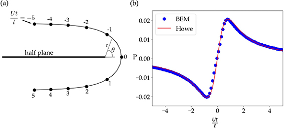
Figure 2. Sound produced by vortex motion near a half plane. (a) Vortex path round the trailing edge of a half plane. The closest position of the vortex to the body  occurs at
  (b) Acoustic response computed by the BEM (blue circles) and from Howe's solution (red line).
Download figure:
Standard image High-resolution imageValidation and verification of the flow-acoustic boundary element framework is detailed in Wagenhoffer et al [43]. A brief recapitulation of the validation follows. Following the experimental work of Booth [44], a vortex is released upstream of a NACA 0012 airfoil, with a chord of c = 0.2032 m. The vortex advects in a freestream of speed  m s−1 with a circulation of
  m2 s−1 at a vertical displacement of
  from the foil centerline (cf figure 3). The experiment was performed in a fluid medium with a speed of sound of
  m s−1 and density ρ = 1.225 kg m−3. The problem schematic at the top of figure 3 depicts how the acoustic response was recorded in front of the airfoil at
  . A comparison of the experimental work of Booth, the matched asymptotic solution by Kao, and the coupled flow-acoustic BEM is shown in figure 3. A similar qualitative response is observed in the matched asymptotic method and the flow-acoustic BEM. The experimental acoustic response produces a signal with more fluctuations, but the responses share similar trends and order of magnitude responses.
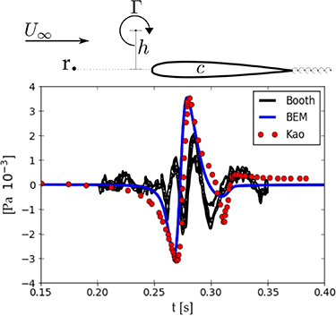
Figure 3. Acoustic emission due to a single vortex advecting past a NACA 0012 airfoil. The schematic denotes the vortex circulation Γ, chord length c, observation point r, freestream velocity  , and offset heights h for the validation cases. The acoustic response at
  is observed 100 chord lengths in front of the foil. The experimental result of Booth [44] is shown as black lines, the matched asymptotic solution of Kao [41] is shown as red circles, and the result of the coupled potential flow and transient acoustics BEM put forward in this work is shown as a blue line.
Download figure:
Standard image High-resolution image3.3. Acoustic emission from biological swimming
Many fish swim by undulating their bodies and oscillating their caudal or tail fins, which are in many cases responsible for the majority of their thrust production [2, 45]. A common and simple representation of a biological swimmer is to neglect the body and only consider the caudal fin as a combined heaving and pitching hydrofoil [46], which is also the case in the present study. Fish-like locomotion via a traveling wave is shown in figure 4(a). The motion of the rear of the foil is tracked and then treated as a discrete propulsive foil, which is denoted in the figure as a solid black body. Figure 4(b) shows how a combined heaving and pitching motion of a rigid body is used as a proxy for the entire traveling wave system. The rigid body pitches about its leading edge, as that is where it would be connected to the fish.
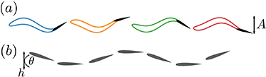
Figure 4. Use of a pitching/heaving foil as a proxy to undulatory locomotion. Illustration (a) shows a period of a traveling wave undulating across a NACA 0012 airfoil. The trailing edge of the foil is modeled as a separate entity that acts as a proxy to the caudal fin of a fish. The schematic (b) tracks the motion of the 'caudal fin' separated from the body as a function of pitching and heaving.
Download figure:
Standard image High-resolution imageThe heaving and pitching motion and the peak-to-peak amplitude of the foil are described by


where f is the frequency of motion, t is time, and h0 and θ0 are the maximum heaving amplitude and maximum pitching angle, respectively. The phase delay between heave and pitch signals is  . The peak-to-peak amplitude is
  , and
, and  is the time at which the foil reaches its peak amplitude. Given
  and θ0, h0 can be calculated by a nonlinear equation solver. Normalizing
  and
and  by
by  produces the identity

Supposing a non-dimensional peak-to-peak amplitude  , the ratio of the heaving and pitching amplitudes is solely described by the non-dimensional heave-to-pitch ratio
  . A purely pitching foil has a value of
  , a purely heaving foil has a value of
  , and
, and  represents a combined heaving and pitching motion where half of the total amplitude comes from pitching and the other half comes from heaving. All other values in the range
  represent combined heaving and pitching motions. The chord-based reduced frequency
  is the non-dimensional quantity that describes the unsteadiness of the prescribed swimming motion.
Figure 5 shows a typical reverse von Kármán wake structure of a foil operating at  ,
,  , and
, and  . The spacing of the wake is dictated vertically by the amplitude of motion and horizontally by the freestream speed and the frequency. The ratio of the vertical spacing to horizontal spacing results in the Strouhal number,
  . The example wake in figure 5 has a Strouhal number of
  which is within the range of typical fish swimming of
  [5, 47, 48]. The acoustic pressure presented for the remainder of this work is non-dimensionalized by dynamic pressure,
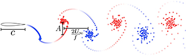
Figure 5. Typical wake of an unsteady swimmer in this study. Wake of a foil after several cycles of motion for the values of  . A foil of chord c is placed in a freestream flow at speed
  . The vertical spacing of the vortices in the wake are described as a function of the amplitude
  and the horizontal spacing is a function of freestream speed and frequency,
  , for half of a cycle of motion.
Download figure:
Standard image High-resolution imageThe flow-acoustic BEM is used to study how variations in the non-dimensional amplitude, reduced frequency, and non-dimensional heave-to-pitch ratio alter both the acoustic emissions and the hydrodynamic forces on the body. The ranges of variables and parameters used in the current study are presented in table 1. The range of Strouhal numbers in the simulations is  . The reduced frequencies and Strouhal numbers in the current study cover the ranges associated with typical fish swimming [5, 48] and also extend to regions where biological systems may perform fast starts or rapid turns [2].
Table 1. Input variables and parameters used in the present study.
| Input variables: |

|

|
| ||
| Input parameters: |
 m s−1 m s−1
| ρ = 1000 kg m−3 |
 m s−1 m s−1
| c = 1 m |
4. Results
Figure 6 presents the near-field transient acoustic pressure over a period of motion ( ) for a foil with parameters of
  ,
,  , and
, and  . The acoustic pressure is determined at discrete points on circles with radii of two to five chords away from the mid-chord of the foil at rest. A vertically-oriented pressure dipole is generally observed. The position of the maximum acoustic pressure shifts from the front to back as the effective angle of attack increases, as seen in the snapshots from
  . The sign change of the dipole strength at snapshots (g) and (n) correspond to the change in effective angle of attack going from positive to negative and negative to positive values, respectively. Snapshots (g) and (n) also exhibit a transient acoustic pressure field with quadrupolar directivity, having two of its lobes directed behind the foil. The work of Khalid et al [49] that the reduced frequency is the controlling feature for the direction of the acoustic dipole-axis. Figure 6 shows a slight tilting of the acoustic near-field dipole, but the response was not significant enough to be of interest and trends of a period of motion were examined, the tilting was found to be averaged out.

Figure 6. Transient near-field acoustic pressure of a typical swimmer. The non-dimensional near-field acoustic pressure P is shown for a foil operating at  ,
,  , and
, and  over a period of motion
  . The acoustic pressure is found at discrete points set around circles centered about the mid-chord of the foil at rest. The circle radii range from two to five chord lengths.
Download figure:
Standard image High-resolution imageFigure 7(a) shows the acoustic response at a single observation point 50 chords above the foil with a heave-to-pitch ratio of  , a reduced frequency of
  , and over the entire range of amplitudes used in the current study. As expected, the pressure fluctuates harmonically in time with the same frequency as the foil motion. For fixed heave-to-pitch ratio and reduced frequency, the amplitude of the acoustic pressure response increases with the amplitude of motion. A directivity plot of the root-mean-square (RMS) pressure (PRMS) over three motion cycles for various reduced frequencies is shown in figure 7(b). Regardless of the motion parameters selected, a dipole directivity is always observed. Moreover, the peak acoustic pressure can be observed to also increase with an increase in the reduced frequency. Since all of the variables produce self-similar dipole acoustic responses, the peak RMS acoustic pressure can be used as the single metric to describe the acoustic field. The peak pressure can then be scaled by the dynamic pressure:

Figure 7. Transient and root-mean-square (RMS) acoustic pressure levels of a typical swimmer. (a) Transient acoustic pressure response of a foil undergoing a combined heaving/pitching motion with  ,
,  , and various amplitudes. The acoustic pressure is determined at the position 50 chords above the leading-edge of the foil and shown for three cycles of motion. (b) RMS acoustic pressure PRMS from a foil undergoing a combined heaving/pitching motion with
  ,
,  , and various reduced frequencies. The acoustic pressure response is computed on a circle 50 chord lengths from the leading edge of the foil and is averaged over three cycles of motion. The dipolar acoustic directivity is observed for all kinematic parameters considered.
Download figure:
Standard image High-resolution imageFigure 8 presents the non-dimensional peak acoustic pressure for a purely pitching foil ( ), a combined-motion foil with equal amplitude contributions from pitching and heaving (
 ), and a purely heaving foil (
 ). The global maximum in the peak acoustic pressure is found at
  ,
,  , and
, and  , which represents the upper bounds of all of the parameters being explored. However, the minimum in the noise production does not occur at the minima of the parameter set: the minimum noise occurs at
  for fixed values of amplitude and reduced frequency. A purely heaving foil produces higher acoustic pressures than a purely pitching foil, except for
  . The combined heaving and pitching foil emits a weaker acoustic pressure signal than either purely heaving or pitching foils for all combinations of reduced frequency and amplitude of motion. Figure 8(b) overlays the Strouhal number on the peak acoustic pressure, showing that in general an increase in Strouhal number results in an increase in the peak RMS acoustic pressure for a fixed swimming motion
  , even though the isolines of St and
  are not precisely aligned. Therefore, the noise level trends are not driven solely by changes in the Strouhal number.

Figure 8. Peak acoustic pressure for (a) a purely pitching foil ( ), (b) a combined heaving/pitching foil (
 ), and (c) a purely heaving foil (
 ) as a function of reduced frequency and amplitude of motion. Isolines of Strouhal number overlay the acoustic pressure contours in (b).
Download figure:
Standard image High-resolution imageAn increase in either the reduced frequency or the amplitude of motion will result in an increase in acoustic pressure, but the motion type of the foil can lead to lower values of acoustic pressure. In fact, a pressure minimum is observed for a combined heaving and pitching motion for all combinations of reduced frequency and amplitude examined in this study. Figure 9 presents a map that shows the  value leading to the lowest noise production for a given
  and
and  . A purely heaving or pitching foil never produces the lowest acoustic pressure. For
  the quietest swimming is produced by pitch-dominated swimming motions (
 ). Only for low reduced frequencies of
  do heave-dominated motions (
 ) produce the quietest swimming, and this
  value is independent of the amplitude. Lines of constant St are also marked on the figure, which denote the typical range of St for swimming animals [47]. From this map it can be seen that for swimming animals operating with low reduced frequencies (
 ) their noise production is minimized if they utilize heave-dominated swimming kinematics. Swimming animals with higher reduced frequency (
 ) minimize their noise production if they utilize pitch-dominated swimming kinematics.
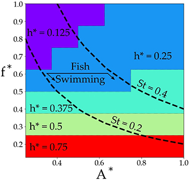
Figure 9. Map showing for a given  and
and  which
which  value leads to the lowest noise production.
Download figure:
Standard image High-resolution imageThe potential flow solver also can solve for the associated performance characteristics of these oscillating foils. The force acting on the foil is defined by  , where Pflow is the pressure from the flow solver as opposed to the acoustic pressure,
  is the local outward normal vector, and
  is the foil surface. Since the potential flow method is inviscid, the forces on the foil arise only from its external pressure distribution. The power consumption of the oscillating motion is calculated as the negative inner product of the force vector and velocity vector of each boundary element, i.e.
  . The time-averaged coefficients of lift, thrust, and power may be defined as
where Fx
and Fy
are the integrated streamwise and transverse components of the force on the foil, respectively. The efficiency is also defined as  . In addition to the time-averaged coefficient of lift, the maximum coefficient of lift will also prove to be a useful metric and is defined by
Figure 10 presents a comparison of the peak RMS acoustic pressure  , the maximum coefficient of lift
  scaled by a factor of 1000 and the absolute value of the time-averaged coefficient of lift
  scaled by a factor of 20. These quantities are shown as functions of the Strouhal number and non-dimensional heave-to-pitch ratio. The lift metrics were scaled in order to make the plots the same order of magnitude. It can be seen that the peak RMS acoustic pressure and the maximum coefficient of lift follow the same trend for increasing
  and
and  . It can also be observed that the peak RMS acoustic pressure does not follow the same trend as the time-averaged coefficient of lift. Not surprisingly, the maximum lift coefficient provides a better correlation with the peak RMS acoustic pressure than the time-average coefficient of lift. In light of this finding, the maximum coefficient of lift
  may be used as a proxy metric for comparison of the relative acoustic emissions between oscillating hydrofoils.
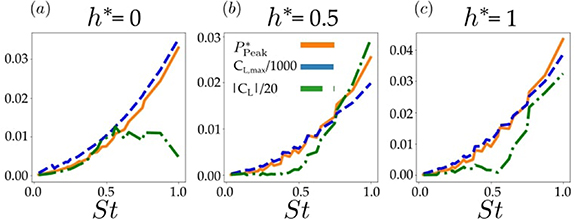
Figure 10. Comparison of lift metrics with peak acoustic pressure as a function of  and
and  . The plots show the peak RMS acoustic pressure
  , maximum coefficient of lift scaled
  , and the absolute value of the time-averaged coefficient of lift
  scaled by a factor of 20. Subfigure (a) is a purely pitching foil,
  , (b) is a combined heaving and pitching motion with
  , and (c) is a purely heaving foil,
  .
.
Download figure:
Standard image High-resolution imageFigure 11 presents a comparison among the coefficients of thrust and power, efficiency, and the peak RMS acoustic pressure. The thrust production increases with increasing  ,
,  , and
, and  . In figure 11, regions of negative coefficient of thrust (and the corresponding regions of coefficients of power, efficiency, and the peak RMS acoustic pressure) are excluded from the contour plots shown. The power consumption also increases with increasing
  and
and  ; however, as
  increases the power decreases to a minimum and then increases. This result indicates that combined heaving and pitching motions use less power than purely pitching or heaving motions for a fixed
  and
and  . The efficiency results show global peaks around
  ,
,  for all
  . Since the
  , the highest efficiencies occur for the lowest swimming Strouhal numbers. Most fish swim with
  [47] making it difficult to reach the highest levels of efficiency, even with
  . The optimal
  to maximize efficiency will vary, depending upon the Strouhal number of the particular swimming animal or biorobotic device.

Figure 11. Comparison of acoustic and hydrodynamic metrics. The rows correspond to the peak acoustic pressure, coefficients of power and thrust, and the efficiency. The columns correspond to different  values. Each contour plot is presented as a function of
  and
and  .
.
Download figure:
Standard image High-resolution imageA novel flow-acoustic BEM was developed to compare the performance and noise of a biopropulsor. The acoustic pressure generated by the foils studied can be simplified as compact systems, where the dominant factor affecting the acoustic pressure is the pressure force acting on the body surface [50]. This pressure force can be accurately modeled as a function of the lift coefficient [51], which is in turn correlated with the power consumption of the foil [52]. These relationships explain the similar trends between the peak acoustic pressure and the power coefficient, as shown in the top two rows of figure 11. Interestingly, the peak acoustic pressure does not follow the same trends as the thrust or efficiency. Furthermore, the absolute coefficient of lift is consistently greater than thrust for all scenarios, which further supports the vertical acoustic dipole and the correlation between the peak RMS acoustic pressure and the maximum coefficient of lift.
These results highlight that when the power needed to move the foil is minimized, then there is also a minimum amount of energy that can be converted into noise, leading to the quietest acoustic signatures. In contrast, there is a trade-off between operating at maximum propulsive efficiency and minimizing the noise production. Furthermore, the thrust increases as the swimmer moves from a pure pitching to a pure heaving swimming motion, which requires more power and produces a louder acoustic signal.
5. Conclusion
An integrated, two-dimensional flow-acoustic boundary element solver is developed to predict the noise generated by the vortical wake of rigid foils in motion. The vortex-particle wake computed by the potential flow boundary element solver furnishes the input for the transient acoustic boundary element solver via Powell's acoustic analogy. This one-way flow-acoustic coupling is validated against experimental and analytical results for the acoustic emission of a vortex gust encounter with an airfoil.
The coupled potential flow-acoustic method is used to investigate the performance and acoustic emission of a heaving and pitching hydrofoil. The hydrofoil is subjected to varying non-dimensional frequencies, amplitudes, and heave-to-pitch ratios that encompass the parametric range of most swimming and maneuvering animals. All combinations of these variables examined in this work produce a similar dipole acoustic response, where the maximum sound pressure levels occur directly above and below the foil. Foils in purely pitching or purely heaving motions are found to be noisier than foils that operate with a combined heaving and pitching motion. In fact, for fixed reduced frequency and amplitude there exists an optimal heave-to-pitch ratio,  , that minimizes the noise production. The numerical model indicates that most swimming animals would minimize their noise production by using heave-dominated swimming motions. As the reduced frequency increases past the regime of swimming animals, a transition to pitch-dominated swimming motions minimize the noise production. Moreover, the correlation between the maximum coefficient of lift and the peak RMS acoustic pressure for all combinations of reduced frequency, amplitude, and heave-to-pitch ratio corresponds to the acoustic dipole response. Consequently, the trends in the coefficient of power are well-correlated with the trends in the peak RMS acoustic pressure for swimming motions with
  . This result supports the conclusion that swimming with low power consumption and a low acoustic signature can be achieved together. In contrast, it is discovered that there is a trade-off between swimming with high propulsive efficiency and a low acoustic signature. These insights seek to further our understanding of swimming in nature and could aid in the design of high-performance, quiet BAUVs.
Acknowledgments
The authors gratefully acknowledge financial support from the National Science Foundation under Grants 1805692 (J W J) and 1653181 (K W M), the Office of Naval Research under MURI Grant N00014-08-1-0642 (K W M), and a Lehigh CORE grant (J W J, K W M).
Data availability statement
The data cannot be made publicly available upon publication because they are not available in a format that is sufficiently accessible or reusable by other researchers. The data that support the findings of this study are available upon reasonable request from the authors.
Appendix: Potential flow BEM validation and verification
The potential flow BEM presented in this work is a two-dimensional derivative of the three-dimensional method described by Willis et al [31]. A comparison of the BEM solution to analytic and numerical works is performed to ensure accuracy of the method presented. Theodorsen [53] solved analytically for the fluid-dynamic lift and moment acting on a flat-plate foil undergoing harmonic pitching and heaving motions under the assumption of a planar wake. Garrick [54] used these results to predict the time-averaged thrust and efficiency of pitching and heaving motions, as well as trailing-edge flap motions. Leading-edge flap actuation has been described in an extension to the pitch, heave, and trailing-edge flap motions of the analytical results of Garrick [55]. Furthermore, computational fluid dynamic simulations of rigid and deformable thin airfoils have been previously compared to the analytic works of Garrick and Theodorsen [56, 57].
The first validation case is against Garrick's theory. In the numerical simulations, a 2%-thick tear drop foil is subjected to a purely pitching motion of amplitude  about the leading edge.
First, convergence studies on the number of boundary elements and time-steps are performed for a reduced frequency  . Figure A1(a) shows spatial and (b) temporal convergence for time-averaged coefficient of force. The inset images detail the percent change (%Δ) of the time-averaged value as the number of elements or time steps per period of motion double. The spatial convergence is conducted for a fixed temporal resolution of 150 time steps per period. The inset of figure A1(a) shows the
  difference in the force when changing from 128 to 256 elements. The temporal convergence study uses a fix number of 256 body elements. It can be seen in figure A1(b) an
  change in force when increasing from 128 to 256 time steps per period of motion. All of the simulation results previously presented use 150 time steps per period of motion and 256 boundary elements to define the discrete body. Wagenhoffer et al [11] details convergence studies of the acoustic BEM and compares results to analytic solutions to show that the selected spatial and temporal values of the potential flow solver will also result in converged acoustic results.
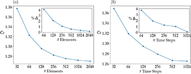
Figure A1. Spatial and temporal convergence of potential flow BEM. (a) Plots the time averaged coefficient of force as the number of boundary elements on the body doubles for a fixed number of time steps.
Download figure:
Standard image High-resolution imageNext, validation via comparison of Garrick's theory to the solution of the solver in section 2.1 for varying reduced frequencies is detailed. Theodorsen defined lift as

and aerodynamic moment as,
where
The required power to sustain the foil motion is  The coefficient of thrust from Garrick [54] was corrected by Jones et al [58] to be
where F and G are the real and imaginary parts of the Theodorsen lift deficiency function,  and a is the position of the pivot point measured from the mid-chord in half-chord intervals. Rotation about the leading edge corresponds to
  .
.
Figure A2 compares the potential flow BEM results against the theory of Garrick for three different reduced frequencies that encapsulate the range of reduced frequencies used for the study in section 3.3. The figure shows the BEM solution matching well to the thin-airfoil theory results over one cycle of motion.

Figure A2. Comparison of BEM solution with solution of Garrick. Shown is a comparison of the solution of section 2.1 to the theory of Garrick [54] for a purely pitching foil. From left to right are increasing values of reduced frequency, 
![$[0.25, 0.5, 1]$](https://content.cld.iop.org/journals/1748-3190/18/4/046011/revision2/bbacd59dieqn176.gif) . From top to bottom are comparisons of the coefficient of lift
. From top to bottom are comparisons of the coefficient of lift  , coefficient of thrust
  , and coefficient of power
  , respectively. In each plot the dashed blue line is the solution of the potential flow method and the solid green line is the theory of Garrick (A.3).
Download figure:
Standard image High-resolution imageThe theory of Garrick is applicable to low-amplitude motion, and additional validation against large amplitude motions is necessary to give confidence in the potential flow solver. The work of Pan et al [33] developed a BEM to investigate leading-edge separation of heaving and pitching foils, but that is not necessary for the work presented here as we assume that the flow remains attached over the propulsive surface being studied. In the work of Pan et al, thrust and efficiency are found for heaving and pitching foils without leading-edge separation for a range of Strouhal numbers and maximum angles of attack  . Figure A3 shows good agreement between the method presented here and the work of Pan et al for a heave-to-chord ratio of 0.75 and
  over
over  .
.

Figure A3. Comparison of the numerical results of the potential flow solver in section 2.1 with the numerical solutions by Pan et al [33]. A combined heaving and pitching motion with a heave-to-chord ratio of  reaching maximum angles of attack of 15∘ (left) and 35∘ (right) are performed over Strouhal numbers ranging from 0.25 to 0.4. The results are compared with respect to the coefficient of thrust
  (top) and efficiency η (bottom). The blue squares represent the work of Pan et al and the yellow circles represent potential flow solver in this work.
Download figure:
Standard image High-resolution image