

Abstract
A general formalism is derived describing both dynamical and energetic properties of a microscopic Feynman ratchet. Work and heat flows are given as a series expansion in the thermodynamic forces, obtaining analytical expressions for the (non)linear response coefficients. Our results extend previously obtained expressions in the context of a chiral heat pump.
Export citation and abstract BibTeX RIS

Original content from this work may be used under the terms of the Creative Commons Attribution 4.0 license. Any further distribution of this work must maintain attribution to the author(s) and the title of the work, journal citation and DOI.
1. Introduction
The Feynman ratchet is a celebrated example of a thermal engine [1]. Designed to illustrate the second law of thermodynamics, it is capable to extract useful work from a heat flow between two thermal reservoirs at different temperatures. The engine consists of two rigidly connected parts, a ratchet and pawl at one end of a rotational axle, and vanes at the other end. Each part is immersed in a surrounding gas, and collisions between the gas particles and the device cause a random rotational motion. The shape of the ratchet introduces a rotational asymmetry which leads to a systematic rotation in a certain direction [2], and is driven by the exchange of heat from the hot to the cold reservoir. Using this rotation for example to lift a weight against the force of gravity, the whole setup can deliver useful work. On the basis of hand-waving arguments, Feynman claims in his Lectures on Physics that the engine is capable of operating at Carnot efficiency. It was realized later [3] that the efficiency inevitably has to be lower, as the engine is at all times in simultaneous contact with the two heat reservoirs, resulting in a heat leakage.
A microscopic analysis of the dynamics and energetics of the original engine has proven to be notoriously difficult. In part this is caused by the unavoidable recollisions of the gas particles with the engine giving rise to correlations. Various approaches have been considered to circumvent these difficulties, for example by modeling the collisions by Langevin noise (e.g. [3, 4]) or by considering a discrete setup, e.g. [5, 6]. An alternative approach was developed by Van den Broeck and co-workers in a series of papers in which they meticulously stripped down the engine to its basic constituents [7–11], see also [12]. Considering ideal gases and convex engine parts (which replace the vanes, ratchet and pawl) an exact microscopic description is derived which is centered around the stochastic time evolution of the (angular) velocity of the device. Analytical expressions for the average velocity are obtained in the form of a series expansion in  , the mass ratio between gas particles and device. Even in such an ideal situation, the interplay between the geometry and the collisions is intricate and it is not at all obvious in which direction the engine will turn. A description of the energetics was obtained by adding a torque [13, 14]. In those papers the work and heat flows were derived from expressions of the average velocity in the linear regime and making use of the Onsager symmetry. The purpose of the present work is to go beyond the linear regime by setting the heat and work variables on the same footing as the angular velocity. Such an extended framework allows to calculate the average (and higher moments of) work and heat up to any order of the thermodynamic forces.
The paper is organized as follows. Section 2 introduces the microscopic Feynman ratchet and describes the dynamics of the engine as the result of the external torque and collisions with the gas particles. Section 3 extends this framework by incorporating both work and heat variables. The main results are presented in section 4, clarifying the influence of the geometry on the motion of the rotor. Finally, we briefly conclude in section 5.
2. Microscopic Feynman ratchet
The original Feynman ratchet was constructed by using a ratchet and pawl on one end of a rigid rotational axle and a set of vanes on the other end. Because of the spatial complexity of such a construction, colliding gas particles are very likely to collide with the various engine parts more than once. This introduces correlations, and hence a memory, making analytical calculations overwhelmingly complicated. In order to eliminate such recollisions, and in effect make individual collisions to occur independently, we reduce the setup to its essence [7]. The purpose of the vanes is to allow transfer of energy from the gas particles to the engine and vise versa. The ratchet and pawl set-up introduces a spatial asymmetry which ensures a difference between clockwise/anti-clockwise rotation of the engine. A conceptually simple construction with these properties is shown in figure 1(a). It consists of two objects rigidly connected by the rotational axis. For such a construction recollisions can be reduced strongly (so that they can be neglected in a subsequent analysis) by requiring (i) the shape of each object to be convex and (ii) the total mass M of the engine to be much larger than the mass m of the gas particles. The first requirement is purely geometrical and ensures that a gas particle is directed away from the object after colliding. The second requirement ensures that a particle, again after collision, is not caught up by the engine. Each object is surrounded by an ideal gas at a certain temperature and density. In the context of a heat engine one of the surrounding ideal gases is labeled as the cold reservoir (sub- or superscript  in the calculations below) and the other one is then the hot reservoir (sub- or superscript
  ). A rotational asymmetry is implemented by shaping the objects asymmetrically with respect to their points of rotation (see figure 1(b)), and by arranging them in an asymmetric fashion with respect to each other. Finally the last ingredient is a weight mounted on the rotational axle which exerts a constant torque τ.
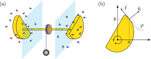
Figure 1. (a) Sketch of the system under consideration: the engine consists of two convex objects rigidly connected by an axle, which serves as the fixed rotational axis. Mounted along the axle is a weight, which is lifted as a result of the collisions of the gas particles with the convex objects. (b) Each convex object is homogeneous along the rotational axis, which allows for a two dimensional analysis. Shown is a top view of the object, indicating the geometrical parameters necessary to describe the collisions with the gas particles.
Download figure:
Standard image High-resolution imageBy construction, the whole engine has only one degree of freedom, namely the rotation around the connecting axle. Its dynamical state is thus fully described by the instantaneous angular velocity ω. In time this velocity changes either due to random collisions of gas particles with any of the two convex objects, or due to the action of the external torque. The effect of the latter is deterministic and described by

where I is the total moment of inertia around the rotational axis of the whole engine.
Quantifying the effect of collisions is more elaborate. Before we start let us set the scene as follows. The surfaces of the convex objects and the gas particles are taken to be smooth, so no tangential forces occur during collisions. As a consequence, collisions of gas particles with the objects' sides which are oriented perpendicular to the connecting axle do not affect ω. Additionally we take the convex rotors to not vary in shape along the direction of the rotational axis, as seen in figure 1(a). Hence collisions with the engine can be analyzed in an effective two-dimensional setup. In order to calculate the effect of a collision, we only need to consider a two-dimensional convex object as sketched in figure 1(b). It is free to rotate around a fixed axis, which is orthogonal to the plane of the object. In that plane we choose a fixed coordinate system with origin located a the center of rotation such that the z-axis coincides with the rotational axis. The orientation of the x and y axis is arbitrary. The instantaneous angular velocity is therefore  . The velocity
  of an arbitrary point
  on the surface of the object is
  . The orientation of the surface at a point
  is specified by the angle ϕ between the x-axis and the tangential unit vector
  . The normal to the surface pointing outward is
  .
.
We now consider a gas particle with mass m and (pre-collisional) speed  as it hits the surface of one of the objects
  at position
  which moves with (pre-collisional) velocity
  . For analyzing this collision we need to consider the total mass M and total moment of inertia I around the rotational axis of the engine as a whole, i.e. of both convex rotors taken together, because they are rigidly connected. The post-collisional velocities (labeled with a prime
  within this section) can be calculated on the basis of the following conservation laws [14, 15]. First, taking the collisions to occur instantaneously, so that the external torque does not affect ω during the collision, the angular momentum along the z-axis is conserved,
  . Second, as there are no tangential forces the tangential velocity of the gas particle is conserved,
  . Third, total energy is conserved which, together with the first two conditions, is equivalent to the condition that the normal component of the relative velocity changes sign,
  . These three conditions uniquely determine the post-collisional velocities,


for which the following quantities are introduced:


Note that the first two parameters, the mass ratio ε and the radius of inertia RI
, are global properties of the engine, whereas the third quantity gα
contains information on the geometry (see figure 1(b)) of the specific part of the engine which is hit by the gas particle in one of the reservoirs and therefore carries the subscript  .
.
Knowledge of the post-collisional velocities as a function of the pre-collisional ones allows to derive the probability per unit time  for the angular velocity to change from ω to a value in the infinitesimal interval
 ![$[\omega^{^{\prime}},\omega^{^{\prime}}+\mathrm{d} \omega^{^{\prime}}]$](https://content.cld.iop.org/journals/1742-5468/2023/4/043202/revision1/jstatacc64eieqn21.gif) due to collisions of gas particles with the convex object in reservoir
due to collisions of gas particles with the convex object in reservoir  :
:
This expression is explained as follows. First there is the integral over the object's one-dimensional surface Sα
which adds up the contributions from all possible points of impact. For each point of impact, the Dirac-δ function picks out those velocities  of the incoming gas particles which lead to the required change
  in angular velocity. The Heaviside-function Θ ensures that the gas particle is moving toward the rotating object. The likelihood for a collision with that specific velocity depends on the properties of the ideal gas in the reservoir
  that enter the equation via the particle density ρα
and the Maxwell-Boltzmann distribution
that enter the equation via the particle density ρα
and the Maxwell-Boltzmann distribution  at temperature Tα
. As this distribution is Gaussian the velocity integrals can be done explicitly and one obtains the expression
at temperature Tα
. As this distribution is Gaussian the velocity integrals can be done explicitly and one obtains the expression
Finally, since the collisions in the hot and cold gas reservoir occur independently of each other, the contributions from the two convex objects simply add up, such that the total rate for transitions of the angular velocity from ω to  is
is  .
.
Having established the transition rates, cf equation (5), together with the deterministic evolution due to the torque given by equation (1), it is straightforward to write down the Master equation describing the time evolution of the probability density 
Instead of solving this equation for  directly, we use a different approach by focusing on the moments of the distribution
  ,
,

Using these moments, the master equation can be transformed to the equivalent (infinite) set of evolution equations [12, 15]:

Here we introduced the so-called jump moments

for the each of the reservoirs  . The equations for the first two moments are


Since there is no approximation involved in deriving (8), these set of equations is fully equivalent to the master equation (6), and is equally difficult to solve analytically. We thus solve (10a
), (10b
) only in the stationary limit, and resort to using an expansion in the small parameter  . An outline of the procedure is given in the
and

where we introduced the friction coefficients [14, 15]

The symbol  (for
(for  ) denotes a average of
  , defined in equation (3c
), over the surface of the object in reservoir α
3
,
, defined in equation (3c
), over the surface of the object in reservoir α
3
,

Figure 2 demonstrates that the theoretical prediction equation (11) for the average angular momentum agrees remarkably well with molecular dynamics simulations of our construction of the Feynman ratchet.
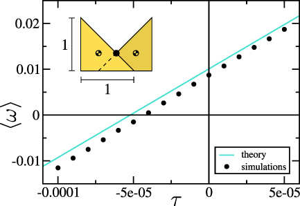
Figure 2. Average rotational speed  as a function of the torque τ: comparison between theory, equation (11), and simulations. Simulations use an event-driven molecular dynamics code with a fluctuating number of point-like gas particles: each convex object is surrounded by a 'simulation box' containing an ideal gas, which is maintained in equilibrium at specific density and temperature by extracting and injecting gas particles through the box walls at the appropriate rates and velocities; see [15] for more details. The error bars for the numerical data are smaller than the symbol size. Inset: Side-view of the system, cf figure 1. The two objects are isosceles right triangles, arranged in a mirror-symmetric way. The filled dot tags the common axis of rotation (with
  ), the two patterned dots represent the center of masses of the two triangles. The system parameters are: M = 20, m = 1,
  ,
,  ,
,  ,
,  ,
,  . Per data point, the simulations tracked about
  collisions in the cold reservoir, and about
  in the hot reservoir.
Download figure:
Standard image High-resolution image3. Energetics and thermodynamics: general framework
Having established the dynamics of the angular velocity ω, via the master equation and corresponding transition rates, we now add the thermodynamic quantities into the framework. In the context of the ratchet system from figure 1 these quantities are heat  and
and  and work W. We define them as positive if delivered to the system. All energy exchanges are mediated by the rotational movement of the engine, and the conceptual simplicity makes a clean distinction between heat and work straightforward. At a momentary rotational speed ω, the rate of work (power) delivered by the external torque is given by

The exchange of heat with the reservoirs is due to the instantaneous collisions of the engine with the gas particle. As each collision is elastic, the kinetic energy change of the imparting gas particle is fully transferred to the rotational energy of the engine. Hence, upon a collision with a gas particle in reservoir α
 that changes the angular velocity from ω to
  , the amount of heat received from the reservoir is given by the corresponding change of kinetic energy

It is clear from these definitions that, while work and heat are fluctuating random variables as they depend on ω, energy conservation is fulfilled at the level of individual trajectories. Our main goal is to analyze the thermodynamic properties of the engine by calculating the lowest order moments  ,
,  , and
, and  .
.
The first step is to incorporate the new quantities as extra variables into the Master equation. The full state is then given by the combined set of variables ω, W and Qα
, where  can be chosen to represent either of the reservoirs. The time evolution of the probability density
  is
is
Compared to equation (6) there is an extra term related to the (deterministic) evolution of W. Moreover, upon a collision one has to keep track of the reservoir, i.e. a collision in reservoir α induces a corresponding change of Qα
, while collisions in the other reservoir (denoted by  ) only change ω. Integrating out the W and Qα
dependence leads to equation (6).
) only change ω. Integrating out the W and Qα
dependence leads to equation (6).
As before, instead of solving the master equation, we turn our attention directly to the moments. The time-evolution of any moment of the quantities of interest ω, W and Qα can be calculated according to

where the function f denotes an arbitrary combination of its arguments. The evolution equations for the lowest order moments of work and heat are then

and

A straightforward calculation yields

which simply expresses conservation of energy. One notices that the equation for the heat depends only on the jump moments of ω. This is a direct consequence of the fact that the stochasticity of the heat Qα
is determined solely by the stochasticity of ω. The expression in equation (20) is obtained from the master equation, equation (17), by multiplying it with Qα
and integrating over all variables ω, Qα
, W. This reduces the equation to  , where
  depends on both ω and
  according to equation (16). In order to express this integral in terms of the jump moments, equation (9), we rewrite
  in powers of
  , i.e.
  ; from this, equation (20) directly follows.
4. Energetics and thermodynamics: results and discussion
The explicit expressions for work and heat quickly become unwieldy and, apart from the already introduced ε expansion, we consider an additional expansion in terms of the so-called thermodynamics forces. These forces appear naturally when looking at the entropy production. From now on we focus on the stationary operation of the machine for which  , where the dot denotes the time-derivative.
The entropy production rate in the reservoirs is given by the combined heat dissipation

Eliminating one of the heat flows in favor of the work (cf conservation of energy) and noting that  allows to reformulate this entropy production into the following two alternatives

There is a priori no preference to choose one over the other, and so we choose to symmetrize by taking the arithmetic mean

This expression is easily cast into the familiar bilinear form

after identifying the two thermodynamic forces

and fluxes

As both fluxes depend on the thermodynamic forces, a series expansion leads in lowest order to the well-known Onsager coefficients


The off-diagonal elements fulfil the Onsager symmetry  .
.
Introducing the reference temperature

allows to substitute τ,  and
and  as
as

Finally we are in a position to give the expressions for work and heat in terms of the relevant thermodynamic forces. These are obtained by a series expansion in both
ε and the thermodynamic forces X1 and X2 (see the
The expressions for the heat are
and
where we defined the thermal velocity

Conservation of energy  follows immediately upon inspection.
The above expressions are the central result of this work. They express the first moments of thermodynamic quantities in the form of series expansion in both ε and the thermodynamic forces X1 and X2, and incorporate in all detail the geometry of each part of the engine. Figures 3 and 4 compare these results, equations (32a )–(32c ), with molecular dynamics simulations of the ratchet construction. The approach taken here allows to go well beyond the thermodynamical linear regime. Although the algebraic calculations quickly become tedious and cumbersome, they are straightforward and easily achievable using a symbolic computation software tool.
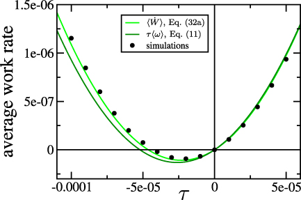
Figure 3. Average rate of work as a function of the torque τ: comparison between theory and simulations. The error bars for the numerical data are smaller than the symbol size. The system, and the simulation setup, are identical to the one in figure 2. As theoretical predictions we show  from equation (32a
) (expressed as a function of τ using
from equation (32a
) (expressed as a function of τ using  , see equation (31)), and
  with
with  given in equation (11). Recall that equation (32a
) is the second-order expansion of
given in equation (11). Recall that equation (32a
) is the second-order expansion of  in the thermodynamic forces X1, X2.
Download figure:
Standard image High-resolution image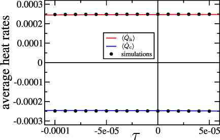
Figure 4. Average rate of heat as a function of the torque τ: comparison between theory equations (32b
), (32c
) (expressed as a function of τ using  , see equation (31)) and simulations. The error bars for the numerical data are smaller than the symbol size. The system, and the simulation setup, are identical to the one in figure 2. We note that the average entropy production rate in the reservoirs, equation (22), corresponding to the shown heat rates is essentially constant; it varies by about 1% around the value
  within the displayed range of external torques.
Download figure:
Standard image High-resolution image
Our approach extends the findings of [14]. In that work the authors considered an identical setup as shown in figure 1 with the purpose to construct a chiral heat pump. In such a setup the external torque is used to drive a heat flow from the cold to the hot reservoir. The analysis of the device was done in the linear regime, making use of Onsager symmetry to complete the off-diagonal elements, without deriving them independently. However, as explained in [14], the external torque not only induces a cooling flux, but also frictional heating in each reservoir. Since it is proportional to  , this frictional heating in fact is of second order in the torque, hence
  . A consistent in-depth analysis of the chiral pump inevitably must go beyond the linear regime. Our explicit results beyond the linear regime confirm the heuristic approach presented in [14], but also reveal the appearance of additional non-linear terms in
  and
and  .
.
As an application of our results, we focus on the efficiency of the microscopic Feynman ratchet. In the context of a heat engine, this efficiency is defined as the ratio of work over input heat,

To see how this efficiency behaves upon varying the forces we write  and
and  , focusing for definiteness on the lowest orders where a, b, c and d can be read of from equations (32a
) and (32c
). It is clear that
, focusing for definiteness on the lowest orders where a, b, c and d can be read of from equations (32a
) and (32c
). It is clear that  equals zero for either
  (no external torque, and consequently no work) or
  , also known as the stopping force. In this case the torque exactly cancels the average angular velocity such that
  . However, even without net rotation when
  and hence
  , there is still a steady entropy production given by
  . Only when
  does the setup behave as a heat engine. Keeping X2 fixed, it is straightforward to prove that the delivered work is maximal when
  (see also [16–18]). Setting
  we find for the efficiency:

with

Notice the presence of the factor  implying A
 . Expressing TX2 in terms of the Carnot efficiency ηC
yields
. Expressing TX2 in terms of the Carnot efficiency ηC
yields

with the last approximation being valid for small temperature differences. We can conclude that the efficiency of the Feynman ratchet evaluated in the limit  is just a small fraction of the Carnot efficiency. The reason we find an efficiency well below Carnot is related to (i) heat leakage and (ii) our expansion in the mass ratio
  . The expressions for the heat rates, equations (32b
) and (32c
), have identical linear terms with opposite signs. Hence, these terms represent heat transfer from the hot to the cold reservoir, directly contributing to the heat leakage. Only differences at nonlinear order quantify the average work rate. In addition to its expansion in the thermodynamic forces this average work rate, being proportional to
. The expressions for the heat rates, equations (32b
) and (32c
), have identical linear terms with opposite signs. Hence, these terms represent heat transfer from the hot to the cold reservoir, directly contributing to the heat leakage. Only differences at nonlinear order quantify the average work rate. In addition to its expansion in the thermodynamic forces this average work rate, being proportional to  , furthermore scales with
  (see the third term in equation (11) and also [14]).
5. Conclusion
A unified framework is developed which treats the dynamical and thermodynamic variables of the microscopic Feynman ratchet on an equal footing. This allows for a detailed and systematic investigation of the thermodynamic performance. Explicit expressions are given for the lowest order moments of all the variables in the form of a series expansion in both  and the thermodynamic forces. As a result it becomes possible to investigate the engine's performance in a systematic way beyond the linear regime.
Acknowledgments
R E acknowledges financial support from the Swedish Research Council (Vetenskapsrådet) under Grant No. 2020-05266. Nordita is partially supported by Nordforsk. B C acknowledges financial support from the Research Foundation—Flanders (FWO) under Grant No. K226922N.
Appendix: ɛ -expansion
We now outline the ɛ-expansion that allows to obtain stationary solutions for the evolution equation (8) of the angular velocity moments  . The approach followed here is a generalization of the one presented in [15] to include (i) two reservoirs at different temperatures and (ii) the external torque τ.
To start we recall the collision rule (2a )

which shows that change in velocity  due to collisions is of order ɛ2. Hence for small ɛ the transition rates
  vanish rapidly for increasing
  . Apart from collisions, ω also changes due to the torque. In order for both these changes to be of order ɛ2 we rescale the torque

Finally, we note that M, through the angular momentum I, also appears implicitly in the velocity ω, as anticipated from the equipartition principle  where T is the reference temperature defined in equation (30). Therefore, we switch to the dimensionless quantity Ω, defined as:

In terms of Ω, equation (8) becomes

with  and
and  the rescaled jump moments whose explicit expression reads:
The function  is Kummer's confluent hypergeometric function [19] defined as the series

where  is the Pochhammer symbol

Expanding the rescaled jump moments in ɛ and inserting the result into (A4) leads to an infinite set of coupled linear equations for the moments  of the following form

with coefficients cnm
depending on the various parameters of the system, including for example ɛ, densities, temperatures, geometries etc. A time-independent solution,  , for this infinite set of coupled equations for the moments is obtained by formally writing each moment in (A8) as a series expansion in ɛ,

and solving for the coefficients up to the desired order in ɛ. Transforming back to the original variables ω and τ, plugging in  and using the definition for
  given in equation (14) leads to the expressions equations (11) and (12).
Once the moments are obtained, the calculation of  ,
,  and
and  as given in equations (32a
)–(32c
) follows directly. For
as given in equations (32a
)–(32c
) follows directly. For  it suffices to substitute
  and further expand in the thermodynamic forces. The expressions for
  and
and  are obtained from equation (20) by first expanding the RHS in ɛ, substituting for the moments, and then again a final expansion in the thermodynamic forces.
Footnotes
- 3
Note that this definition differs from the definition we used in [15] by a factor of unit length representing the total 'surface' of the object.