


Abstract
Plasma filaments have been measured with alkali beam emission spectroscopy in the plasma edge, divertor island, and scrape-off layer of Wendelstein 7-X. Due to the high intensity of a 1–2 kHz plasma mode, a new, correlation based conditional averaging algorithm was used to search for filaments in the signals. With that method, effects of different magnetic configurations and density levels on filament properties are observed. In configurations where the islands are small and do not play an important role for the connection length topology, filaments behave similar to tokamaks. In contrast, in configurations with larger magnetic islands and more complex connection length profiles, filaments behave quite differently, for instance they may or may not appear in the inner side of the divertor island depending on the plasma parameters. Coupling between the filaments and lower frequency events are also showed. The role of filaments in the global and local particle transport is briefly discussed.
Export citation and abstract BibTeX RIS

Original content from this work may be used under the terms of the Creative Commons Attribution 4.0 license. Any further distribution of this work must maintain attribution to the author(s) and the title of the work, journal citation and DOI.
1. Introduction
Filaments or blobs [1] are well known phenomena in many types of magnetically confined plasmas. These field-aligned structures can transport heat and particles from the plasma edge to the Scrape Off Layer (SOL). Their extension along the field lines can be even in the order of ten meter, while their perpendicular size is in mm–cm scale. In tokamaks filaments with positive density perturbation are seen to be born in the edge plasma, close to the last closed flux surface (LCFS). Although the question of blob generation is not decided yet, according to 2D models they are produced by interchange instability on the low field side of tokamaks. Due to the nonlinear growing phase of such instability filaments can detach from the main plasma. In these density perturbations a charge separation is created by curvature and grad B drift. The resulting electric field causes an outward  drift while, for negative perturbations remaining in the edge plasma (holes) it causes an inward
  drift. These phenomena are considered to be a major particle and heat transport process from the plasma edge to the SOL.
The electric field in filaments can be influenced by possible connections to material surfaces. The two fundamental cases are the sheath-limited and inertial ones. In the former regime currents flowing along the field lines are connected on the target plates, which reduces the charge separation, and thus the electric field and filament velocity. This occurs at short connection length and at low collisionality. In contrast to that the inertial regime can occur at high density, and/or long connection length. In that case the charge separation in filaments is limited by currents that are perpendicular to the magnetic field lines. Filaments can have much stronger polarization in that state, and thus higher velocity. Radial filament size may also depend on these regimes [2], and transition from the sheath-limited to the inertial state are often linked to the appearance of a density shoulder, thus filaments can have a significant influence over the density profile in the SOL.
Filament dynamics are considered to be mostly understood by quasi-2D situations, where the curvature and shearing of magnetic field lines change slowly along the filament. This is true in tokamak limiter plasmas and in poloidal divertor configurations in the far SOL region. However, in situations where there is strong magnetic shear, for instance in tokamak divertor plasmas around the X-point, it can distort the filaments [3]. In such situations a 3D approach of filament modeling is inevitable [4].
First results of filament observations on Wendelstein 7-X have been reported using fast video cameras [5], alkali beam emission spectroscopy (ABES) [6], and Langmuir probes [7]. However, essential questions about their dynamics in the divertor island are still open. It is a difficult task to understand filaments in W7-X due to the complicated three-dimensional geometry [8] of the device, and particularly the topology of the divertor island [9]. Here in the SOL the normal magnetic curvature varies considerably along field lines. Such environment for filaments is just starting to be addressed with simulations [10]. Numerical studies [11] claim that filaments can exist and propagate outward in the presence of a non-uniform curvature drive as long as the field-line averaged curvature is negative. This behaviour is enabled by the high conductivity along the field lines which effectively averages polarization.
The present paper describes filament properties based on ABES signals in the edge, in the divertor island and in the SOL using a new conditional averaging (CA) algorithm, and other statistical methods. It compares the effects of different magnetic configurations and density profiles. Evidence of interrelations between filaments and events with longer timescales [12] are also documented.
2. Experimental set-up
The ABES system [13] on W7-X includes an 50 kV neutral sodium beam [14] injected on the equatiorial plane (see figure 1) of the device at  toroidally, and observed perpendicularly to the beam [15]. It goes through the SOL, the divertor island o-point, and the plasma edge. Beam atoms are excited by collisions with plasma particles, of which electrons have the largest contribution, thus the atoms emit light at the sodium doublet line (
 nm) among others during their transition to the ground state. The intensity of that line is measured by 32 Avalanche Photo Diode (APD) and 8 Multi-Pixel Photon Counter (MPPC) detector channels along the beam. The MPPC channels are the outermost ones. These 40 detectors are observing the beam from a vertical position, providing
  cm spatial resolution in the radial direction and integrating light for 4 cm toroidally. Spatial smearing along the beam due to the lifetime of the excited state is 1 cm in the far SOL [13] and further reduced by collisional processes in the island and edge plasma. The beam diameter is about 2 cm, thus the diagnostic is sensitive mainly for perturbations which have at least that poloidal size. The temporal resolution is set by 500 kHz analog bandwidth and 2 MHz sampling rate. Depending on plasma configuration and location the signal to noise ratio can reach up to 50. As it was shown in [16] the limited spatial resolution also means that the diagnostic is sensitive only to the low frequency part of the filament spectrum.
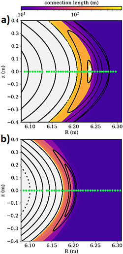
Figure 1. Poincaré plots of W7-X magnetic surfaces at  toroidal angle with connection lengths indicated by the color code at each position on the R–Z plane. The green circles denote the measurement points of the APD (and MPPC) channels along the beam. The two plots are referring to different magnetic configurations: (a) standard, (b) high iota.
Download figure:
Standard image High-resolution imageThe plasma of Wendelstein 7-X is bounded in one cross-section by different number of magnetic islands (often referred to as divertor islands) depending on the magnetic configuration. In high iota configuration  in a divertor island, and that means there is one island, which wraps around the main plasma four times. The low iota magnetic configuration is similar, but with the exception that
  in the islands. Therefore, in that case the island wraps around the main plasma six times. There is a great difference in magnetic topology between the previous cases and the standard configuration, where
  in a divertor island: in this case the main plasma is bounded by five individual magnetic islands. Due to these facts, if one starts to follow a field line, it takes at least four or six toroidal turns to end up at a similar poloidal position in high or low iota configurations, while in standard configuration it is only one toroidal turn. However, the divertor islands also have their own iota profile, thus even in standard configuration there will be some displacement in the island after a toroidal turn. Therefore, in the low and high iota configurations it is highly unlikely that a filament is so long that it may interact with itself, while in standard configuration it might be possible if the filament is at least one toroidal turn long [6]. This way the complex magnetic topology of Wendelstein 7-X may affect the dynamics of filaments.
As it can be seen in figure 1, in standard configuration on the outer side of the island the connection lengths to the divertor plates are in the order of tens of meters, while on the inner side, between the o-point and the separatrix of the main plasma, it is a few hundred meter. There are closed flux surfaces around the o-point of the island—such extreme connection length profile may influence the filament properties greatly. In contrast to that, in high iota configuration the connection length is a continuous and monotonic function from the far SOL to the main separatrix, furthermore the island is narrow—thus the magnetic configuration is more similar to a typical tokamak Scrape-Off Layer—plasma edge area from that point of view.
3. Signal processing methods
At low edge density (
 ) the sodium beam light intensity is approximately proportional to the local electron density, as the beam ionization is low. Thus under such condition the beam light fluctuations can be used as a proxy for electron density fluctuations. As the beam enters regions with higher electron density, the ionization starts to dominate and the measured light will not be proportional to the local electron density anymore. That only holds for signals measured deeper than maximum of the light profile. The utilization of an electron density reconstruction algorithm is inevitable in such cases [17]. However, this algorithm was found unsuitable for the study of small perturbations as the global fitting introduces non-local response. Therefore, light signals were used in most cases, and the method became useful for density reconstruction of the CA results. Furthermore, the light signals were only used to the depth where the beam emission maximum is. Figure 2 shows the mean of measured ABES light profiles during the discharges used in the present paper.

Figure 2. Mean of ABES light profiles measured during non-transient phases of the plasma at the analyzed plasma parameters and magnetic configurations. The dashed lines denote the separatrix, the dotted line denotes the o-point of the island.
Download figure:
Standard image High-resolution imageThe beam was modulated by a given frequency in order to allow the separation between the light emitted by the beam and the background. During certain discharges (for instance 20 181 018.026) the modulation period time was 20 µs, thus by taking the average light for different periods, and subtracting the background signal values from the ones which were measured with an active beam, one may gain a beam light signal with 20 µs temporal resolution. During other discharges the modulation period was 150 ms. To gain a beam light signal with the same temporal resolution, the data measured at beam on was integrated to 20 µs. The background signal level was calculated by averaging the signal for beam-off periods and linearly interpolating between them. The beam light signal was calculated by subtracting the interpolated background values from the beam-on signals. By choosing such method, background fluctuations were neglected. However, the background is small compared to the active signal (the signal-to-background ratio—SBR was always between 2 and 10 on every channel), thus it is a well-founded approximation.
A first order, recursive bandpass temporal filter with 3.2–10 kHz band was used to separate the frequency range of filaments from other phenomena (see figure 3). Above 10 kHz the power spectra of the ABES system contains the QC-mode [6, 18] at certain radial positions. Furthermore, the SNR decreases with the frequency. The reason behind the lower limit was an attempt to separate the signal from a 1–2 kHz mode [19]. However, that can not be perfectly done due to the fact that such filters do not have a sharp cut off frequency, and the mode is also not at a fixed frequency, thus, some power remains from the mode even after one applies the filter, as it can be observed in figure 3. Sharper cut bandpass filters were found to produce more distortion in the signals. Separation of the low frequency modes is absolutely necessary, without it the conditional averaging algorithm cannot be used.

Figure 3. Autopower spectra of an ABES light signal before and after a first order recursive bandpass temporal filter with 3.2–10 kHz bandwidth was applied on it. The signal was measured during discharge 20 181 018.003 in the time interval of ![$t = [2.14, 4.61]$](https://content.cld.iop.org/journals/0029-5515/64/1/016017/revision2/nfad0af7ieqn12.gif) s.
s.
Download figure:
Standard image High-resolution imageAs one can see in figure 4, the utilized narrow bandwidth filter may distort the shape of the events: before filtering there can be seen a positive event, and after filtering it is a sinus-like oscillation. It may be regarded as a positive event as well as a negative event, if one wish to perform conditional averaging based only on the signal levels after the application of a filter. This may lead to different, false results, when one calculates the average filament shape and rates.

Figure 4. Illustration of the distorting effect of 3.2–10 kHz bandwidth, first order, recursive filters on an ABES signal from discharge 20 181 018.026.
Download figure:
Standard image High-resolution imageTo solve the problem a correlation based conditional averaging (CA) algorithm was developed [20]. Firstly, it filters the signal with an 3.2–10 kHz bandpass filter as above. Secondly, it calculates the C(t) correlation between this filtered signal and a Gaussian pulse G(t) filtered with the same bandpass filter in a sliding time window:
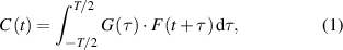
where F(t) denotes the filtered signal and T is the length of the interval belonging to the filtered Gaussian.
The sign of the Gaussian depends on the sign of the events searched for. The algorithm then selects the intervals where  (σ is the standard deviation of C(t) in the whole processed time interval), and stores the middle point of the intervals as time of the events. The program executes that process for Gaussians

with 


 50 µs parameters, then it merges the lists of chosen events. After that the algorithm averages the unfiltered signals around the selected times with a chosen length (which might be different from T). The interval selection is based on a single detector signal, but the averaging is done on other signals from other radial positions as well, thus the radial filament shape can be determined. If one is not interested in the lower frequency structures which are in phase with the filaments, then the program may perform a parabola fit (to the edges of the averaged signal) and subtraction on the CA results to separate the filament itself. In the present article these parabola fits were only performed when 2 ms long intervals were chosen around the event. Such parabolic trend removal could be viewed as an effective filter on the CA result, which does no interfere with the event selection process. This algorithm is similar to a wavelet transformation [21], however, wavelets are not useful if one aims to search for blobs and holes separately. A similar method was published [22] with iteration for the shape of G(t).
The reason behind the chosen s parameters is the following. The Fourier transform of the Gaussian in (2) is also a Gaussian:

where  and
and  . The maximum of the latter Gaussian is at zero frequency, however, it has significant intensity in the frequency spectrum up until the half of its maximum
  . Thus, one can say that a relevant part of the power spectrum of the Gaussian with parameter s remains after filtering if 3.2 kHz
  kHz. This approximately holds for the
 ![$s = [18,50]$](https://content.cld.iop.org/journals/0029-5515/64/1/016017/revision2/nfad0af7ieqn22.gif) µs interval, as it corresponds to
µs interval, as it corresponds to ![$f_{HM/2} = [3.75,10.41]$](https://content.cld.iop.org/journals/0029-5515/64/1/016017/revision2/nfad0af7ieqn23.gif) kHz.
kHz.
The above described CA algorithm, using the signal of a given channel, provides an average filament (or some other event, if the filaments are not the dominant phenomena). On such result (provided that parabolic trend removal was not performed) one may use the fast electron density reconstruction algorithm [17] to gain information about the density of filaments. The procedure involves performing the density calculation on the sum of the CA light profiles and the mean light profile. From the result the mean density profile is subtracted to yield the density perturbation by the conditionally averaged filament.
An example for CA results, and their reconstructed density profiles can be seen in figure 5. The reconstruction algorithm is not accurate enough for the exact determination of filament shape, but its result can be used for filament density intensity estimation by taking the difference between the maximum of the reconstructed event and the mean density value for the discharge at the given radial position.
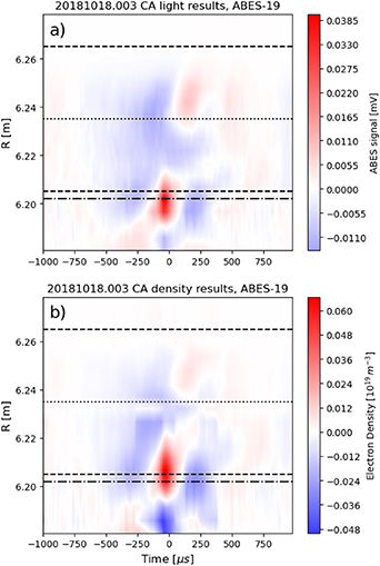
Figure 5. Conditional averaging results on ABES signals in discharge 20 181 018.003: (a) shows the conditionally averaged light signals, (b) shows the electron density reconstruction. A parabolic temporal trend removal on the result was performed, but only after the density reconstruction. The dashed lines denote the separatrix, the dotted line denotes the o-point of the island. The dashed–dotted is the channel on which the algorithm searched for events, whose radial coordinate is R = 6.2018 m. The algorithm found 299 events per second.
Download figure:
Standard image High-resolution image4. Results
In present paper electron-cyclotron wave heated (ECRH) discharges in the standard and high iota configuration were analyzed. Table 1 lists the main discharge parameters. The heating power was changed in discharge 20 181 018.020, therefore the two parts with different heating powers were analyzed separately.
Table 1. Analyzed discharges and the corresponding magnetic configurations denoted with the rotational transform in the island, ECRH power levels, line integrated densities, respectively. Further notations: '1'. stands for the first half of the discharge (![$t = [1,6]$](https://content.cld.iop.org/journals/0029-5515/64/1/016017/revision2/nfad0af7ieqn24.gif) s), while '2'. stands for the second half of the same discharge (
s), while '2'. stands for the second half of the same discharge (![$t = [7,12]$](https://content.cld.iop.org/journals/0029-5515/64/1/016017/revision2/nfad0af7ieqn25.gif) s).
s).
| Discharge | ιisl | PECRH |

|
|---|---|---|---|
| 20 180 912.014 |

| 3.47 MW |
 m−2 m−2
|
| 20 181 018.003 |

| 4 MW |
 m−2 m−2
|
| 20 181 018.020 1. |

| 4 MW |
 m−2 m−2
|
| 20 181 018.020 2. |

| 2.2 MW |
 m−2 m−2
|
| 20 181 018.026 |

| 4.5 MW |
 m−2 m−2
|
4.1. Standard configuration
4.1.1. Correlation in the island.
In a recent article [6] it was shown that there is a correlation with time delay between ABES signals measured at the plasma edge and outer side of the divertor island in discharge 20 181 018.003 (see table 1) in the frequency range of plasma filaments (1.6–10 kHz). This phenomenon can be seen in figure 6. It is challenging to explain such correlation between the filaments due to the fact that these radial regions are not connected by field lines. Furthermore, the time lags between filaments in the two regions indicate much higher radial propagation velocity for the filaments than expected.
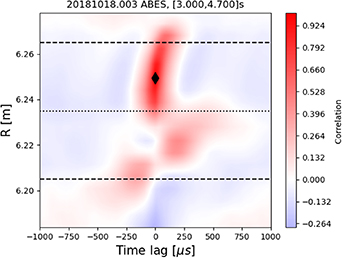
Figure 6. Correlation between signals coming from different radial positions in discharge 20 181 018.003. The signals were filtered with a 1.6–10 kHz first order, recursive filter. The dashed lines indicate the island separatrix, while the dotted one shows the o-point of the island. The diamond symbol marks the reference point.
Download figure:
Standard image High-resolution imageWe may take into account that the above introduced 1–2 kHz mode [19] has the highest intensity in standard configuration with low line integrated density, it modulates the density in the whole island, and it possibly has a peak up to 2.5 kHz. Figure 7(a) shows the coherency of ABES light signals between points at plasma edge and outer side of the island, while figure 7(b) shows the coherency between points at the inner and outer side of the island. Comparing these, one may see that the coherency is significant up to 3 kHz in both cases, thus the correlation in figure 6 must come from that frequency range. In contrast to that, as we can see in figure 7(c), if one examines two signals which come from the outboard side of the island, the coherency is significant up to 7 kHz. If the coherence is only significant in the f < 3 kHz range between channels on the outboard side and the LCFS, then it is possible that it is the effect of the 1–2 kHz mode, and that correlation between the LCFS and the outboard side in figure 6 has no connection to filaments.

Figure 7. Coherency between light signals measured in time interval ![$t = [3,4.7]$](https://content.cld.iop.org/journals/0029-5515/64/1/016017/revision2/nfad0af7ieqn37.gif) s in discharge 20 181 018.003 at (a) the outer side of the island and the edge (b) the outer and inner side of the island (c) two locations in the outer side of the island. The absolute value of the error was taken as significance.
s in discharge 20 181 018.003 at (a) the outer side of the island and the edge (b) the outer and inner side of the island (c) two locations in the outer side of the island. The absolute value of the error was taken as significance.
Download figure:
Standard image High-resolution image4.1.2. Filament properties in standard configuration at low density.
In the case of discharge 20 181 018.003 (see table 1) we applied the CA algorithm to a dataset of 1.2 s usable beam time. In that experiment the electron density was smaller than  m−3 along the beam in the SOL according to the reconstructed density profiles, thus, the light signals are sufficient for measuring filaments in the whole divertor island.
In figures 5 and 8 there are CA (searching for positive pulses) results from the outer side on the island and in the plasma edge, respectively. The algorithm did not find filaments in the inboard side of the island. In figure 8 there can be seen significant positive intensity on the inner side of the divertor island and in the plasma edge, but with phase shifts—similarly to figure 6. A reasonable explanation for such structures is that the 3.2–10 kHz bandwidth, first order, recursive filter did not remove the 1–2 kHz mode perfectly, as it can be seen in figure 3. It is close to the region of filaments in the frequency domain, consequently, the CA algorithm could have taken some peaks of the 1–2 kHz mode as filaments. The similarity in time lags between figures 6 and 8 also supports that.
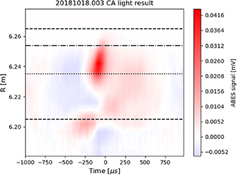
Figure 8. Conditional averaging results on signals measured during discharge 20 181 018.003. A parabolic temporal trend removal on the result was performed. The dashed lines denote the separatrix, the dotted line denotes the o-point of the island. The dashed-dotted is the channel on which the algorithm searched for events. Measurement points along the beam, and number of found events in the signal: R = 6.2538 m, 336 s−1.
Download figure:
Standard image High-resolution imageFigure 8 shows that filaments on the outer side of the island have 2–3 cm radial extension, while based on figure 5 in the edge plasma they have 1–2 cm. Filaments at the edge plasma are also faster events (they have smaller temporal extension). It could be the result of different connection lengths: figure 1 shows that on the outboard side of the island filaments could be in the sheath-limited regime due to the small connection lengths there, thus, their radial velocity should be reduced [1]. On the inner side and close to the inner separatrix the divertor is far along the field lines, which may result in inertial filaments. That means these filaments should have higher radial velocity, which may cause smaller temporal width, as we can see in figure 8. According to [6] the poloidal velocity of filaments in the two regions does not differ significantly. The temporal shifts of the maximum filamentum intensity in the radial direction also indicate higher radial velocity in the high connection length regime, which supports this argument. Nevertheless, the poloidal structure may also contribute to the temporal size of the event, it can also cause apparent radial propagation [23]. However, the poloidal shape of filaments is not determinable by ABES due to the lack of resolution in that direction.
4.1.3. Filament properties in standard configuration at high density.
During the next examined discharge, 20 181 018.026, the line integrated electron density was two times higher than in the previous one, while the ECRH level was almost the same (as one can see it in table 1). At such high plasma density ABES signals provide reliable information about filaments until the o-point of the island according to figure 2. Due to the fact that during this discharge the beam was modulated with high frequency, the analyzed time length of signals is 7.898 s under stationary plasma conditions. Figure 9 shows an example of CA results from this discharge. As it can be seen, these filaments have approximately 2 cm radial extension, but otherwise there is no significant difference comparing to figure 8 except that the intensity of the structure attributed to the low frequency mode is lower.

Figure 9. Conditional averaging result on a signal measured during discharge 20 181 018.026 at radial position R = 6.2538 m. The algorithm found 241 events per second. A parabolic temporal trend removal on the result was performed. The dashed lines denote the separatrix, the dotted line denotes the o-point of the island. The dashed-dotted is the channel on which the algorithm searched for events.
Download figure:
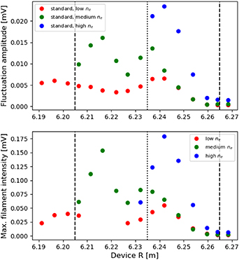
Standard image High-resolution imageIn figure 10 one may compare the filament density, rate and the mean density profile of high electron density discharge 20 181 018.026, and low electron density discharge 20 181 018.003 (we will discuss the medium density experiment in the next subsection). Outside the main plasma separatrix the density is approximately two-three times higher in the former one, which results in filaments with two-three times higher electron density (up to  of the background at their peak). There is no such large difference in the filament rates. Some rate and intensity values are missing in the low density case as the CA algorithm did not find filaments on the inner side of the island.
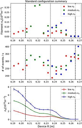
Figure 10. Uppermost figure: maximum filament intensities in the reconstructed density versions of CA results in discharge 20 181 018.003 (denoted by low ne
), 20 181 018.020 in ![$t = [7,12]$](https://content.cld.iop.org/journals/0029-5515/64/1/016017/revision2/nfad0af7ieqn39.gif) s (denoted by medium ne
) and 20 181 018.026 (denoted by high ne
)—further details are in table 1. Middle figure: number of events found by the CA algorithm in the same discharges. Lowermost figure: average reconstructed density profiles for the same discharges in the analyzed time intervals. The error of the showed profiles is the mean of the averaged profile errors, which were estimated by the reconstruction algorithm.
s (denoted by medium ne
) and 20 181 018.026 (denoted by high ne
)—further details are in table 1. Middle figure: number of events found by the CA algorithm in the same discharges. Lowermost figure: average reconstructed density profiles for the same discharges in the analyzed time intervals. The error of the showed profiles is the mean of the averaged profile errors, which were estimated by the reconstruction algorithm.
Download figure:
Standard image High-resolution image4.1.4. Filament dynamics on the inner side of the island.
In discharge 20 181 018.020 (standard configuration) two different ECRH power levels were applied, and in the second half (![$t = [7,12]\,s$](https://content.cld.iop.org/journals/0029-5515/64/1/016017/revision2/nfad0af7ieqn41.gif) ) it was 2.2 MW with somewhat lower integrated density (see table 1). In this time interval low density enables us to use the light signals for filament detection also on the inner side of the island according to figure 2.
) it was 2.2 MW with somewhat lower integrated density (see table 1). In this time interval low density enables us to use the light signals for filament detection also on the inner side of the island according to figure 2.
Figure 11 shows CA results from the island in the above described case. In contrast to previous discharges, here filaments occur in the inboard side of the island as well. Their radial size is 2–3 cm. It is also worth to mention that there is a sharp phase shift, or time lag in the maximum of filaments between channels at R = 6.2267 m and R = 6.2220 m according to figure 11. It might be the effect of the complex magnetic topology of the magnetic island around the o–point: one may end up at a few centimeter distance after a toroidal turn along the field lines based on figure 1. Thus here it is highly likely that a filament may interact with itself while passing through this region, and maybe that causes this time lag.
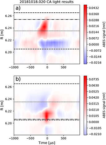
Figure 11. Conditional averaging results on signals measured during discharge 20 181 018.020, time interval ![$t = [7,12]$](https://content.cld.iop.org/journals/0029-5515/64/1/016017/revision2/nfad0af7ieqn42.gif) s. A parabolic temporal trend removal on the result was performed. The dashed lines denote the separatrix, the dotted line denotes the o-point of the island. The dashed-dotted is the channel on which the algorithm searched for events. Measurement points along the beam, and number of found events in the signal: (a) R = 6.2538 m, 269 s−1, (b) R = 6.2065 m, 308 s−1.
s. A parabolic temporal trend removal on the result was performed. The dashed lines denote the separatrix, the dotted line denotes the o-point of the island. The dashed-dotted is the channel on which the algorithm searched for events. Measurement points along the beam, and number of found events in the signal: (a) R = 6.2538 m, 269 s−1, (b) R = 6.2065 m, 308 s−1.
Download figure:
Standard image High-resolution imageIn figure 10 we can compare the overall results of two plasma parameter settings from the following discharges: the just described second half of 20 181 018.020 (from now on it will be referred as medium density discharge), and the previously examined 20 181 018.003 (see table 1). There are huge differences in the rate and filament density profiles in the inner side of the island. One can observe many quite high density filaments (their density peaks are 5%–25% of the background) there in the medium density discharge, while no filaments were found there in the low density case. A possible explanation for the phenomenon is that the overall higher and steeper density profile results in more filaments with higher density. We already saw evidence in the previous chapter for the latter.
Figure 12 shows electron density profiles from the first and second halves of discharge 20 181 018.020 (see table 1). It is notable that in response to decreasing heating power the electron density decreased in the island, which is in agreement with the reciprocating probe measurements [24]. Given the fact that the intensity and number of filaments in figure 10 imply that they might have an important role in the particle transport during higher density discharges on the inner side of the island, it is possible that filaments carry significant density to the island. It would give an explanation for the relatively larger change in density around the o-point compared to the plasma edge density in discharge 20 181 018.020 (figure 12): less steep density profile in the edge could result in less dense filaments, thus these filaments could carry less particles into the island.
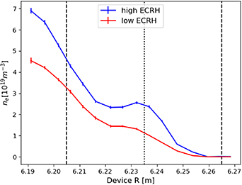
Figure 12. Average reconstructed density profiles in discharge 20 181 018.020 between ![$t = [1,6]$](https://content.cld.iop.org/journals/0029-5515/64/1/016017/revision2/nfad0af7ieqn43.gif) s (denoted by high ECRH),
s (denoted by high ECRH), ![$t = [7,12]$](https://content.cld.iop.org/journals/0029-5515/64/1/016017/revision2/nfad0af7ieqn44.gif) s (denoted by low ECRH). The error of the showed profiles is the mean of the averaged profile errors, which were estimated by the reconstruction algorithm.
s (denoted by low ECRH). The error of the showed profiles is the mean of the averaged profile errors, which were estimated by the reconstruction algorithm.
Download figure:
Standard image High-resolution image4.2. Filament properties in high iota configuration
Discharge 20 180 912.014 was a high iota magnetic configuration experiment (see figure 1) with relatively low line integrated electron density and moderate heating power (as we can see in table 1). The density profile was a monotonically decreasing one in the SOL, as it is shown in figure 13. Here the analyzed time length was 1.8972 s. Figure 13 also shows an example of the CA results from that experiment: 4 cm radially extended filaments were found at every position along the beam where there was a significant amount of electron density. Compared to figure 11 it can be seen that in high iota configuration filaments have a different, less complex radial structure, probably due to monotonically decreasing connection length along the beam (in contrast to the standard configuration—see figure 1). This is consistent with correlation analysis presented in [6].
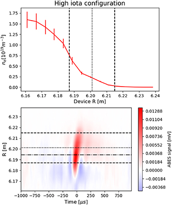
Figure 13. Upper figure: average reconstructed electron density profile in the analyzed time interval in discharge 20 180 912.014. Lower figure: conditional averaging result on a signal measured during the same discharge at radial position 6.1946 m. The algorithm found 338 events per second. A parabolic temporal trend removal on the result was performed. The dashed lines denote the separatrix, the dotted line denotes the o-point of the island. The dashed–dotted is the channel on which the algorithm searched for events.
Download figure:
Standard image High-resolution image4.3. Connection to low frequency events
The previously presented CA method can fit a temporal parabolic function to the two ends of a CA result, and then subtract it. However, by skipping that process, and taking a larger time interval around the filaments, it is possible to observe lower frequency events, modes around them in CA results, as it can be seen in figure 14. The structure of such phenomena clearly depends on the density in the island, and the magnetic configuration (see table 1). Based on its frequency and intensity, what figure 14(a) shows is the Quasi-continuous low frequency edge fluctuation, which had been measured by Rogowski coils [12]. The connection between the low frequency phenomena and the filaments is not clear. As the CA method used in this paper does not rely on signal amplitudes but rather on pulse shape, it is unlikely that these modes appear in the CA results through low frequency signal modulation. Therefore, there is some real temporal correlation between the low frequency events and filaments.
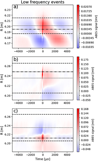
Figure 14. Conditional averaging results on ABES signals. The dashed lines denote the separatrix, the dotted line denotes the o-point of the island. The dashed-dotted is the channel on which the algorithm searched for events. Discharge, measurement points along the beam, and number of found events in the signal: (a) 20 180 912.014 (high iota configuration with low density), R = 6.1945 m, 314 events per second, (b) 20 181 018.026 (standard configuration with high density), R = 6.2477 m, 208 events per second, (c) 20 181 018.020, ![$t = [7,12]$](https://content.cld.iop.org/journals/0029-5515/64/1/016017/revision2/nfad0af7ieqn45.gif) s (standard configuration with medium density), R = 6.2113 m, 288 events per second.
s (standard configuration with medium density), R = 6.2113 m, 288 events per second.
Download figure:
Standard image High-resolution image4.4. Skewness, and its implications on transport
In tokamaks [1] generally the skewness of the probability distribution function of the signal is negative in the plasma edge, reaches zero at the separatrix, and increases up to (at least) 2–3 in the far SOL. The explanation behind it is that there are positive and negative filaments, blobs and holes, which are born around the separatrix. Blobs are propagating outward, while holes are propagating inward due to the sign of their density perturbation which determines their polarization. These movements cause less blobs inside the separatrix and more on the outside, vica versa regarding the holes. That leads to more negative peaks in the signal inside the separatrix, while more positive signal outside which causes the monotonously increasing skewness.
A recent article [7] showed that in W7-X low iota configuration the skewness of Langmuir probe ion saturation current signals is close to zero along the probe path in the SOL, which supported the conclusion that filaments do not move far during their lifetime, and there are blobs and holes as well in the SOL. Thus, filaments do not represent a large perpendicular transport like in the usual case in tokamaks. In the present article we do not use the traditional CA method (like in [7]), instead we utilized the new one which was described above, and we calculated the skewness of the C(t) function. C(t) should have a positive peak for blobs and negative for holes, but should be less sensitive to the low frequency modes which would distort the skewness of the original signal.
In figure 15 we calculated C(t) at each radial location for different Gaussians, then took the skewness of these time series, and averaged these values obtained for the different Gaussians. It is clear that in standard configuration, in the outer side of the divertor island the skewness is close to zero in all cases, but there is a significant increasing tendency in the high and low density discharges. We can also see a maximum in the medium density case in the inboard side, which fits well to the filamentum density profile in figure 10. One must take into account that the skewness values of ABES signals are expected to be lower than the skewness of Langmuir probe signals due to the relatively high signal to (photonic) noise ratio in the former [25]. Therefore, the skewness profiles in standard configuration indicate that not all filaments move only locally during their lifetime.
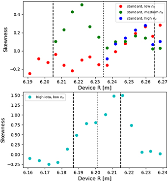
Figure 15. Mean skewness of correlation data between Gaussians and ABES signals filtered to 3.2–10 kHz range. The upper plot shows discharge 20 181 018.026 ( m−2), 20 181 018.020
 ![$t = [7,12]$](https://content.cld.iop.org/journals/0029-5515/64/1/016017/revision2/nfad0af7ieqn47.gif) s (
s ( m−2), and 20 181 018.003 (
 m−2), all of them were performed in standard magnetic configuration. The lower plot shows a high iota configuration discharge 20 180 912.014 with
  m−2.
m−2.
Download figure:
Standard image High-resolution imageFigure 15 makes it clear that in high iota configuration the skewness goes above 1.5 in outboard side of the island, which means that it is dominated by blobs, and these were born deeper in the plasma. Such results point in the direction that the blobs in high iota configuration are more similar to tokamak blobs, and travel large distances during their lifetime.
4.5. Negative events
As it was discussed above, the skewness is close to zero in standard configuration along the beam, which indicates that there should be a balance between positive and negative events. That means there are negative events, possible holes in the SOL. It is straightforward how to apply the CA method for hole searching: if we change the sign of the Gaussians in the algorithm, it is already sufficient. It is equivalent to a search for negative events in C(t) (see (1)). Such results can be seen in figure 16. Figure 16 shows that in many cases negative events are accompanied by positive ones in the SOL, and the amplitude of their minimum suffer a positive time lag along the radial direction outward just as the maximum of positive filaments (see figures 8, 9 and 13). A previous article [6] interpreted that such a time lag in the correlations (see figure 6) is a result of the propagation direction and velocity of filaments. However, knowing that in the CA results we can see negative events accompanied by positive ones with the same time lags, that previous statement is at least questionable, due to the fact that holes in plasmas should propagate inward [1]. One possible explanation for such phenomenon is the following: if the structures are inclined in the radial-poloidal plane relative to the equatorial plane, then their poloidal movement can cause apparent radial propagation [23]. A definite statement on this phenomenon can only be made if poloidally resolved measurement would be available either by side observation [16] on the Sodium beam or by utilizing a quasi 2D BES technique by hopping the beam between two poloidal location [26, 27].
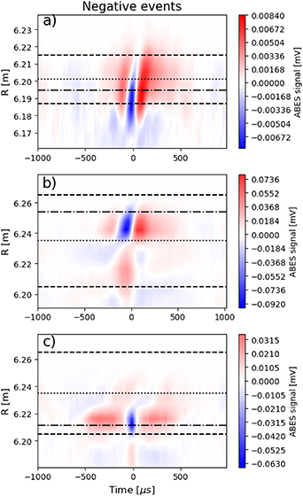
Figure 16. Conditional averaging results on ABES signals (using negative Gaussian). The dashed lines denote the separatrix, the dotted line denotes the o-point of the island. The dashed-dotted is the channel on which the algorithm searched for events. A parabolic temporal trend removal on the result was performed. Discharge, measurement points along the beam, and number of found events in the signal: (a) 20 180 912.014 (high iota configuration with low density), R = 6.1946 m, 268 events per second, (b) 20 181 018.026 (standard configuration with high density), R = 6.2538 m, 199 events per second, (c) 20 181 018.020, ![$t = [7,12]$](https://content.cld.iop.org/journals/0029-5515/64/1/016017/revision2/nfad0af7ieqn51.gif) s (standard configuration with medium density), R = 6.2113 m, 235 events per second.
s (standard configuration with medium density), R = 6.2113 m, 235 events per second.
Download figure:
Standard image High-resolution imageAnother, possible explanation for the coupled positive–negative events could be that the results in figure 16 are false negative events, as the filtered negative Gaussians of the CA algorithm could have relatively strong correlation with the filtered positive events like in figure 4. This could indeed give a contribution to the results. However, in case when this effect dominates, no negative intensity would be seen in the CA results, only two positive ones, as the algorithm does not take the average on the filtered signal. In contrast to that, the negative events in figure 16 have similar intensities as the surrounding positive ones. Nevertheless, according to [16], the holes seen by BES systems can be smaller than the blobs in some cases, and these events are more easily absorbed. This, and the previously described false blob identification process of the algorithm together could provide a reasonable explanation for the seemingly linked positive–negative events in the SOL. The diagnostics detects the holes, however, these are small. Therefore, in the CA algorithm such events are mixed with the largest positive filaments, as the signal is dominated by blobs.
According to figure 17 pure negative events can be found with the CA algorithm in standard configuration in the edge. The inward propagation of the holes should result in more holes than blobs inside the LCFS, which is also observed here (454 vs. 220), and that accounts for the negative skewness at that radial position (see figure 15). This result supports the arguments in the previous paragraph: one can see that at radial positions where holes dominate, they indeed can be observed. Furthermore, the time lag of the correlation maximum in figure 17 indicates inward propagation in contrast to the results in figure 16. However, this cannot be clearly established in the absence of poloidal resolution.

Figure 17. Conditional averaging results on ABES signals (using negative Gaussian) from discharge 20 181 018.003 (standard configuration with low density). The dashed lines denote the separatrix, the dotted line denotes the o-point of the island. The dashed–dotted is the channel on which the algorithm searched for events—it corresponds to radial position R = 6.1911 m. A parabolic temporal trend removal on the result was performed. The program found 454 events per second.
Download figure:
Standard image High-resolution image4.6. ABES-MPM comparison
Wendelstein 7-X has a Multi-Purpose Manipulator [24] diagnostic with reciprocating electric probes mounted on it. The probe head contained a poloidal array of cylindrical probes, and some of them were operated in ion saturation current ( ) mode. The head was located at
  and around
  cm in the cylindrical coordinates of the device, while it was movable in the radial direction. The reciprocating probe head is not connected by magnetic field lines to the ABES measurement points. The probes were installed on the head in two poloidal arrays, where each array is tangential to the flux surface shape.
For the purpose of validation of the results, ABES signals and MPM Isat
measurements are compared briefly. Unfortunately, there were no measurements, when both diagnostics were in operation, and the MPM stayed at one radial position for a sufficient amount of time. For that reason, MPM  signals from discharge 20 181 010.023 with
  m−2 line integrated density, 5 MW ECRH are used for comparison. In that experiment the MPM took radial position R = 6.083 m for two seconds, where the connection length is in the order of 30 m. Three different probes measured
  , two were in one line, the other one was in the other probe line, and the largest distance between two was 2.5 cm. These signals were summed up here simulating the reduced poloidal resolution of the ABES diagnostic (2 cm). From the discharges which have valuable ABES signals, 20 181 018.003 is the closest to the one with MPM data available, they were both performed in standard configuration, the only difference is that during the one with ABES data available the ECRH power was 4 MW. In standard configuration the most similar measurement point to the above described with ABES is at radial position R = 6.254 m (there the connection length was almost the same as above—see figure 1).
Both the number of found events by CA per second, and the average skewness of correlation data are significantly higher for the MPM signals: the number of events were 717 for the MPM and 400 for the ABES, while the skewness was 0.4197 versus 0.1766. Both results point in the same direction: the MPM diagnostic detects more events. A viable explanation could be that summing up the signals of three probe heads does not simulate properly a measurement volume with 2 cm diameter. Which means one can see less filaments with ABES, because it has a different spatial scale, and it is not that sensitive to small density perturbations as the MPM [16].
5. Discussion
The presented events in section 4.1 have several unique properties compared to filaments measured in tokamaks [1]. Therefore, one could argue that these are different phenomena, and these events should not be called plasma filaments. Let us examine the similarities and the differences. Firstly, in tokamak SOL-s the frequency range of filaments is characterized by intermittency and non-Gaussian PDF. In practice it means the skewness of the filtered signal is in the order of 1 and increasing, while the kurtosis is larger than one and increasing as well towards the wall. In our case this tendency is visible on the outer side of the island in the skewness (figure 15), however, it never reaches even 0.6. Moreover, the mean kurtosis value of the signals filtered between 3.2-10 kHz in our radial range of interest varies between 0.88 and 2.54 in standard confuguration, while it is 3.75 in high iota configuration.
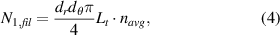
Another way to investigate whether the phenomena in question are filaments or not is to examine the definition of filaments [1]. Firstly, a filament is an event with a monopole ne
which is larger than the RMS fluctuations of the background plasma (its intensity is typically 2–3 σ). According to figure 18, the calculated filament maxima are larger than the local fluctuation amplitudes by a factor of 5–10, thus the first point holds for these phenomena. Secondly, a filament is highly localized perpendicularly to  , it is field-aligned. The radial size of the presented events is 1–3 cm. Correlation between edge filaments measured by ABES and fast video cameras were presented in a previous article [6], which showed the toroidal elongation and poloidal localization of these events. The third point of the definition refers to the the polarization of the filaments, and the fact that their movement is governed by the
  drift. Unfortunately, one cannot measure the electric field with ABES. Nevertheless, the presented positive events possess the characteristic single-peaked shape in density, thus the curvature
  drift should polarize these events. It can therefore be seen that these events meet the general definition of filaments.
Figure 18. Upper figure: fluctuation amplitude profiles of the ABES signals in standard configuration discharges after a 3.2–10 kHz bandpass filter with sharp frequency cut-offs. Lower figure: intensity maximum of filaments averaged by the CA algorithm at the given radial positions.
Download figure:
Standard image High-resolution image
Let us discuss the relation between filaments and low frequency events. One explanation is that the interchange instability (the possible source of blobs) is more sensitive to a steeper density profile. Thus, during any mode or event, which temporary increases the density in the island significantly, more filament arises than without it. Due to that when we are performing a CA, we can observe the low frequency plasma modes in phase with the filaments.
Another, possible explanation could be that these modes are the MHD response functions to the filaments passing through the plasma. It is questionable, because there are examples, when we see the low frequency event after the filament (like in figures 8 and 9), but other times the filament is in the middle of the larger structure (figures 14(a) and (c)). We may mention a third possible explanation: plasma bursts, instabilities often have filamentary structure. It is possible that the CA algorithm triggers for such structures, thus, on average, we see such phenomena around the filaments.
Concerning comparison to tokamak measurements one can see that in high iota configuration the filaments look very similar to the ones observed in tokamaks. In standard configuration on the outboard side of the magnetic island (SOL) there is also some similarity to tokamak filaments, like increasing skewness towards the far SOL in some cases, 1–3 cm radial size, maybe higher radial velocity at higher connection length (based on their temporal extension—see figure 8). Although, the skewness is generally lower in standard configuration.
The presence of filaments on the inboard side of the island in standard configuration is a crucial question as they may play a role in setting the density in the island, and this is affecting divertor operation. The information obtained in various discharges so far is summarized in figure 10. From this it seems that the line integrated (core) density determines whether filaments are present on the inboard side. In this region the density profile has a minimum or more flat than in the edge plasma and the SOL, therefore the interchange mode is less unstable there and filaments are not, or less effectively generated here as it was already shown in [6]. At higher edge plasma density the filaments generated at the steeper pressure gradient in the edge plasma will presumably penetrate deeper into the island, this might be a reason for observing here filaments only at higher density. In such case the density gradient is also higher in the inner side of the island, which is more interchange-unstable than in the low density discharge, thus it is more likely that filaments are generated locally as well. The sum of these two effects may cause the maximum in the filament rate and skewness profiles.
Finally, one can make a crude estimation for the number of particles carried by filaments through the LCFS, therefore, it is determinable whether they play a significant role in global particle confinement or not. By approximating the filament cross-section with an ellipse characterized dr , dθ parameters (referring to the radial and poloidal diameter, respectively), and assuming that they have Lt long toroidal extension, the number of particles carried by a filament is
where  is the average filament density. By assuming the same escape rates and intensity for positive filaments on the whole Low Field Side (LFS) separatrix of the device, one can estimate the particle loss per second due to filament activity:
where R denotes the average number of filaments passing though the separatrix per second, and  is the outer separatrix surface of the main plasma. In this expression the poloidal size of the filaments (which is not measured by ABES) is not present, only data which are determined by our analysis. Let us use the data from discharge 20 181 018.003 for the estimation—in that case, the average density of the filaments at the LCFS was
  m−3, and the number of found filaments was 270 s−1, while their average radial diameter was
  cm. The (effective) outer part of the LCFS is approximately 15.13 m2. Consequently, the number of particles carried by filaments through the separatrix is
  s−1. According to [28, 29], the average particle confinement time was τ ≈ 100 ms during the OP1.2b campaign, while the plasma volume is 30 m3. By assuming
  m−3 particle density, we have
  particle in the device. That means if the particles could only go through the separatrix in filaments, the confinement time would be approximately
  s. We can see that
  , which means the role of filament activity in the frequency range of 3.2–10 kHz is negligible in the global particle transport. This agrees with the result obtained in [6], however, the just performed analysis contains more data and less assumption. Nevertheless, the number of particles in the divertor island is smaller than in the core plasma by orders of magnitude. Consequently, filaments may have a significant role in the local cross-field transport and influence on the density profile, as it is indicated by figures 10 and 12.
6. Conclusions
Field-aligned plasma filaments were observed by ABES diagnostic using a new CA method. The results show that in high iota configuration, in which the connection length along the beam is a continuous function of the minor radius, the filaments are radially extended up to 4 cm, and they are propagating outward. The skewness profile is negative in the edge, changes to positive at the separatrix, and goes up to 1.5 in the island. Furthermore, the average kurtosis value in the investigated radial range is 3.75. These observations indicate that in that configuration the filaments have very similar properties to the ones measured in tokamaks.
In standard magnetic configuration the situation is more complicated. Filaments are born at least at two locations: in the edge and in the outboard side of the island, where the density profile is steep and its gradient is negative, thus it is interchange-unstable. On the outer side of the island filaments have approximately 3 cm radial extent, while in the edge it is 1.5 cm. The edge filaments are also temporally shorter. On the outboard side of the island (SOL) filaments are always present, while on the inboard side they are not seen at low density. A possible reason is that filaments generated in the edge plasma can penetrate deep into the island only if they have high density. This might affect the density level in the island and through that divertor operation as well.
The correlation between filaments in the plasma edge and the outer side of the island [6] is most likely the consequence of the 1–2 kHz mode [19]. However, according to CA results there are time correlations between filaments and other, low frequency events in the island. The shape and intensity of such events depend on the configuration and the density profile.
The signal skewness is lower than in a typical tokamak SOL even considering the limited spatial resolution of the alkali beam diagnostic and the skewness decreasing effect of photonic noise. Related to this, negative events accompanied by positive ones can be observed with seemingly outward propagation in the SOL. The most likely explanation for such phenomenon is that the CA algorithm often takes large blobs as holes, if the holes are relatively small. Thus, if only small holes are present that could lead into averaged positive-negative events in the SOL. However, inside the LCFS, where the skewness is negative, pure negative events were found, which supports the presented explanation, as holes dominate at that radial regime. Thus, it is possible that positive and negative filaments born in most of the SOL as it was stated in [7]. Nevertheless, with our current methods, we cannot see the holes in the SOL clearly using ABES signals.
Acknowledgments
This work has been carried out within the framework of the EUROfusion Consortium, funded by the European Union via the Euratom Research and Training Programme (Grant Agreement No. 101052200—EUROfusion). Views and opinions expressed are however those of the authors only and do not necessarily reflect those of the European Union or the European Commission. Neither the European Union nor the European Commission can be held responsible for them.