


Abstract
Global gyrokinetic simulations of ion temperature gradient (ITG) and trapped electron mode (TEM) in the LHD stellarator are carried out using the gyrokinetic toroidal code (GTC) with kinetic electrons. ITG simulations show that kinetic electron effects increase the growth rate by more than 50% and more than double the turbulent transport levels compared with simulations using adiabatic electrons. Zonal flow dominates the saturation mechanism in the ITG turbulence. Nonlinear simulations of the TEM turbulence show that the main saturation mechanism is not the zonal flow but the inverse cascade of high to low toroidal harmonics. Further nonlinear simulations with various pressure profiles indicate that the ITG turbulence is more effective in driving heat conductivity whereas the TEM turbulence is more effective for particle diffusivity.
Export citation and abstract BibTeX RIS
1. Introduction
The stellarator is increasingly becoming an attractive and promising concept in the quest of magnetically confined nuclear fusion due to its intrinsic advantages of not having a toroidal current, lower levels of MHD activities, steady state operation, and absence of disruptions [1–3]. However, these benefits come at the cost of toroidal symmetry breaking that leads to an increase in the neoclassical transport, and stronger damping of zonal flows as compared to the axisymmetric tokamaks [4, 5]. To mitigate these disadvantages, quasi-symmetry and quasi-isodynamicity concepts have been developed as further optimization of the stellarator configuration [6–8]. Following this trend, the Large Helical Device (LHD) has recently been optimized with a strong inward shift of the magnetic axis to reduce the neoclassical transport to a level of an advanced stellarator [9]. After the reduction of neoclassical transport, the microturbulent transport in the stellarators still remains a major challenge. For example, phase contrast imaging (PCI) of the core plasma fluctuations shows evidence of the ion temperature gradient (ITG) and trapped electron mode (TEM) turbulence in the W7-X stellarator [10]. In a similar way, characteristic signatures of the ITG turbulence [11–14] have been observed in the LHD. Therefore, the presence of microturbulence in stellarators remains a serious challenge and it is of great importance to gain a proper understanding of their nature and dynamics.
Over the past few years, some progress has been made toward gyrokinetic simulations of microturbulence in stellarators. Gyrokinetic flux-tube simulations using GKV code have been carried out extensively in the LHD [15–17], where the reduction of the ITG turbulence due to zonal flow, the role of the zonal flow on the TEM turbulence, and the effects of isotopes and collisions on the microinstabilities in the LHD have been studied. However, the flux-tube simulations do not capture the linear coupling of multiple toroidal harmonics due to the 3D structure of the magnetic field in the stellarators and the secular radial drift of helically trapped particles across flux surfaces.
Hence, a global gyrokinetic simulation study is required to have a better understanding of the microturbulence in the stellarators. The first global gyrokinetic simulations using the EUTERPE code with adiabatic electrons were recently carried out to study the effects of the radial electric field on the ITG turbulence in W7-X and LHD [18]. The gyrokinetic toroidal code (GTC) has been used to carry out the first global nonlinear ITG turbulence simulations with adiabatic electrons in the W7-X and LHD [19]. GTC has also self-consistently calculated neoclassical ambipolar radial electric fields in the W7-X, which were shown to suppress the ITG turbulence more strongly in the electron-root case than the ion-root case [20]. Furthermore, XGC-S [21] and GENE-3D [22] have performed global gyrokinetic simulations of microturbulence in the W7-X using adiabatic electrons. The adiabatic electron model cannot address the effect of kinetic electrons on the ITG turbulence [23, 24], and the excitation of the TEM turbulence [25].
Kinetic electrons were first incorporated in the global gyrokinetic simulations of the W7-X and LHD to study the collisionless damping of zonal flow [26]. Subsequently, GTC simulation with a sufficiently high mesh resolution found a new helical trapped electron mode (HTEM) in the W7-X [27]. Finally, GENE-3D with a reduced mesh resolution has been used in recent work to perform the simulations of the electromagnetic ITG turbulence with kinetic electrons in the W7-X-like plasma [28].
In this paper, we present global gyrokinetic simulations with kinetic electrons of microturbulent transport in the LHD stellarator. The GTC code [29] is employed for this purpose in order to investigate the growth rate, nonlinear turbulent transport, as well as the linear and nonlinear spectra of the ITG and TEM turbulence. ITG turbulence simulations show that the kinetic electron effects increase the growth rate of the most unstable mode and the turbulent transport. GTC simulations indicate that the zonal flow leads to a decrease in the ITG transport levels by the zonal flow, hence the zonal flow acts as the ITG dominant saturation mechanism. The TEM simulations show that the linear eigenmode is localized on the outer mid-plane of the LHD, opposite to the W7-X HTEM localization in the inner mid-plane [27]. However, the self-generated zonal flow is found to have an insignificant effect on the dynamics of the TEM transport. Rather, the inverse cascade of the high poloidal and toroidal harmonics to the lower harmonics is the dominant saturation mechanism. The role of zonal flow in TEM turbulence suppression has been widely discussed for axisymmetric tokamaks [30–37] and has been shown that the zonal flow effects are typically weaker in the TEM turbulence than in the ITG turbulence. However, the strength of the zonal flow in regulating the TEM turbulence depends on detailed plasma profiles and parameter regimes for both tokamaks [37] and stellarators [38]. A comparison of the transport coefficients between different cases for η = 0, 1, and ∞, where η is the ratio of the ion temperature gradient to the density gradient, shows that the ITG turbulence is more effective in driving the heat conductivity whereas TEM turbulence is more effective for the particle diffusivity.
This paper is discussed as follows: in section 2, the three-dimensional geometry and simulation model are presented. In section 3, ITG and TEM turbulence simulations with kinetic electrons are presented. Finally, conclusions are made in section 4.
2. Stellarator geometry and simulation model
Gyrokinetic toroidal code (GTC) is a global 3D code to study the physics of microturbulent transport [25, 39], Alfvén waves [40], energetic particles [41], and radio frequency waves [42] in toroidally confined plasmas. To reduce the particle noise due to Monte Carlo sampling of particle distribution, GTC uses a low noise δf method [43] in which only the perturbed part of the particle distribution is evolved with time. GTC simulations performed in this paper use the non-axisymmetric equilibrium of the LHD stellarator [18] constructed by the ideal MHD code VMEC assuming closed magnetic surfaces [44]. The equilibrium geometry and the magnetic field are described as the Fourier series in both poloidal and toroidal directions on a discrete radial mesh that is equidistant in the toroidal flux. These equilibrium quantities are then transformed to the Boozer coordinates as the Fourier series in the toroidal direction on discrete grid points on the 2D poloidal plane [45]. The 3D quadratic spline interpolation is used in GTC to represent the equilibrium magnetic field and metric tensor on an equilibrium mesh [45]. The 3D LHD equilibrium used in this paper corresponds to the 'outward shifted' configuration and has been used in earlier work for self-consistent GTC simulations [19, 26]. The LHD device has a symmetry with a field period of Nfp = 10, which means all the equilibrium quantities have a periodicity of 2π/Nfp in the toroidal direction. Therefore, for turbulent transport, there are ten drift wave eigenmode families corresponding to the ten field periods. Earlier GTC simulations had found similar ITG growth rates for these ten eigenmodes, each coupling all toroidal n harmonics [19]. The equilibrium magnetic field on the flux surface with ψ = 0.36ψw is shown in figure 1, where ψw is the poloidal flux on the last closed flux surface. Due to the field symmetry of the LHD, one-tenth of the torus is simulated which is represented by the dashed lines in figure 1. The 'eye' in figure 1 indicates the point of view of the following 3D figures.
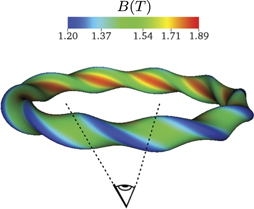
Figure 1. The 3D real space contour plot of magnetic field amplitude on the flux surface with ψ = 0.36ψw.
Download figure:
Standard image High-resolution imageThe field-aligned mesh is used to represent the fluctuating quantities in GTC and provides the maximum numerical accuracy and computational efficiency without making any geometry approximation [39]. As the particles are pushed maximally in the direction of the field lines, the perturbed quantities vary slowly in the parallel direction as compared to the perpendicular to the field lines. So, only a few parallel grid points are required to resolve the particle dynamics in the parallel direction. The 5D-gyrokinetic equation [46, 47] describing the ion dynamics is
where

and
where  is the equilibrium magnetic field at the guiding center position of the particle, B is the equilibrium magnetic field at particle position,
  is the unit vector along the magnetic field, Ωi is the ion gyro-frequency.
  is the particle distribution function with
  being the coordinates of the gyro-center, μ is the magnetic moment of the ion and v|| is the ion velocity parallel to the magnetic field.
  is the
  drift and
  is the magnetic drift velocity. ϕ is the electrostatic perturbed potential, Z and m are the charge and mass of the ion.
To reduce the particle noise, δf method [43] is used, in which the particle distribution function is written as the sum of equilibrium part and the perturbed part as, f = f0 + δf. Writing equation (1) as Lf = 0, where the propagator L can be written as L = L0 + δL, with

and

The equilibrium distribution satisfies L0 f0 = 0 and the perturbed distribution can be calculated as (L0 + δL)δf = −δLf0. An additional dynamical variable, 'w' the particle weight is defined as w = δf/f, that satisfies

The electrostatic potential ϕ is also decomposed into a zonal part and a non-zonal part as  , where the angle bracket
  represents the flux-surface averaging. To consider the effect of kinetic electrons on turbulence, kinetic description of electrons is required. However, being lighter, the electron has a fast parallel motion that puts a constraint on the time step size to be used due to the 'ωH
' mode [48], that, in turn, makes the simulations computationally expensive. To overcome this limitation, the electrons are described by the hybrid model [24] in which the electron distribution function that satisfies the drift kinetic equation, can be written as
represents the flux-surface averaging. To consider the effect of kinetic electrons on turbulence, kinetic description of electrons is required. However, being lighter, the electron has a fast parallel motion that puts a constraint on the time step size to be used due to the 'ωH
' mode [48], that, in turn, makes the simulations computationally expensive. To overcome this limitation, the electrons are described by the hybrid model [24] in which the electron distribution function that satisfies the drift kinetic equation, can be written as
The electron equilibrium distribution satisfies L0
f0 e = 0. To the lowest order, the electron response is adiabatic with  , and the term δhe represents the higher order correction which is nonadiabatic in nature. The non-zonal potential is further expressed as the sum of adiabatic and nonadiabatic parts, δϕ = δϕ(0) + δϕ(1). The nonadiabatic parts δϕ(1), δhe are smaller than the adiabatic parts δϕ(0),
  by a factor of δ, where δ is the fraction of magnetically trapped electrons. The electrostatic potential is obtained from the following gyrokinetic Poisson equation [48]

where  , δne are the ion and electron guiding center charge density, n0 is the equilibrium electron density, and τ = Te/Ti. The term on the left-hand side is the ion polarization term [48]. The gyrokinetic Poisson equation for non-zonal component of the electrostatic potential in the lowest order electron response can be written as

where  is the second gyro-averaged perturbed potential defined as

where  and
and  are the coordinates of particle position and the particle guiding center position respectively and
  is the gyro-radius vector.
  is first gyro-averaged perturbed potential given by

and similarly

is the ion perturbed density at the guiding centers, where α is the gyro-phase. The contribution of '1' in the factor (1 + τ) multiplied to the first term on left-hand side of equation (6) comes from the adiabatic part of the electron density. The particle orbits and fields are updated iteratively in a time stepping sequence. With all field quantities known at kth time step, ion orbits are pushed to (k + 1)th time step using the ion gyrokinetic equation. A finite difference method is used to obtain the lowest order solution of the non-zonal potential from equation (6). The higher order term in the electron distribution which is related to the nonadiabatic electron weight as we = δhe/fe, is calculated from the following first order drift kinetic equation
where  , the gradient operator on ln fe 0 inside the square brackets on right-hand side is taken with v⊥ held fixed. While writing equation (7), the exact perturbed potential δϕ on right-hand side is approximated by the lowest order solution δϕ(0). Also, it is also assumed that the equilibrium pressure gradient scale length is much longer than the perturbation scale length and the wavelength of electrostatic fluctuations is much longer than the electron gyro-radius. Using all the field quantities at kth time step in equation (7), the electron orbits are now pushed from the kth time step to (k + 1)th time step. Using the expansion of electrostatic potential and the electron distribution function, the non-zonal component of electrostatic potential to the first order is obtained from

with  . Equations (7) and (8) are solved iteratively to reach the higher-order depending upon the trapped fraction. Usually, the second-order iteration is sufficiently accurate for typical device parameters. However, the equations for ions are solved only once. Finally, all the particle orbits and non-zonal components of field quantities are updated at (k + 1)th time step and the zonal component of the electrostatic potential at (k + 1)th time step is obtained by solving

The cycle of equations (6)–(9) can be repeated at the next time step. Collisions have been discarded from the present study to focus on the effect of zonal flow on the turbulent study. Since a finite boundary is implemented in the simulations, the energy-conserving boundary condition is implemented in GTC for the particles facing the simulation boundary.
3. Microinstabilities in LHD
Drift-wave instabilities arise in fusion plasmas due to the non-uniformities of the plasma profile. In this section, the microinstabilities responsible for most of the anomalous turbulent transport observed in fusion plasmas, mainly ITG and TEM, are studied in LHD with the GTC code. Various temperature and density profiles are used in order to analyze the different instabilities. Thus, the ratio η = ∇ln Ti/∇ln n will be different for each simulation. In section 3.1, an ion temperature gradient is set to excite the pure ITG turbulence (η = ∞), then in section 3.2 the pure TEM instability can be analyzed when a density gradient is applied (η = 0). Finally, in section 3.3 both density and ion temperature gradients are applied (η = 1) and the resultant turbulent transport is analyzed. The profiles used in the simulations have been chosen to excite these microinstabilities in LHD plasma and are not meant to be the same as experimental profiles or previous gyrokinetic simulations [16, 17]. In the entire study, a uniform electron temperature profile is set and no equilibrium radial electric field is taken into account.
3.1. ITG
As mentioned in section 1, global gyrokinetic simulations of ITG turbulence with adiabatic electrons have been carried out in non-axisymmetric devices as the LHD and/or W7-X stellarators using GTC [19], EUTERPE [49], XGC-S [50] and GENE-3D [22] codes. More recently, GENE-3D performed simulations of ITG in W7-X with kinetic electrons but reduced the mesh resolution to solve the fastest growth rate [28]. Here, we expand the GTC work done in reference [19] by including kinetic electrons in ITG simulations using the model described in section 2.
The plasma profile used for the pure ITG turbulence simulations is shown in figure 2. The on-axis ion temperature is 2 keV, the electron temperature is 1 keV, and the maximum normalized ion temperature gradient is  at ψ ∼ 0.33ψw where the rotational transform is ι ∼ 0.5. The inverse ion temperature gradient scale length is defined as
  , where r is the local minor radius. The dashed black lines represent the simulation domain with ψinner = 0.08ψw, ψouter = 0.7ψw. A uniform density profile is set so η = ∞. After a convergence test, we use 200 radial grid points, 2700 poloidal grid points and nine parallel grid points. The number of particles per cell is 50, the time step size is 0.016R0/Cs
, where Cs
/R0 = 7.82 × 10⁴ s−1 and
, where r is the local minor radius. The dashed black lines represent the simulation domain with ψinner = 0.08ψw, ψouter = 0.7ψw. A uniform density profile is set so η = ∞. After a convergence test, we use 200 radial grid points, 2700 poloidal grid points and nine parallel grid points. The number of particles per cell is 50, the time step size is 0.016R0/Cs
, where Cs
/R0 = 7.82 × 10⁴ s−1 and  is the speed of the ion acoustic wave. To resolve electron dynamics a time step 40 times lower is used. The linear instability threshold for the ITG turbulence is
  .
.

Figure 2. Radial profiles for the equilibrium ion temperature Ti (blue solid line), the electron temperature Te (blue dashed line), normalized ion temperature gradient  (red solid line), used for the simulations of ITG turbulence with η = ∞. The black dashed lines represent the simulation boundary with ψinner = 0.08ψw and ψouter = 0.7ψw.
Download figure:
Standard image High-resolution imageFigure 3 shows the time history of ion heat conductivity (averaged over ψ ∈ [0.19, 0.38]ψw) of the four nonlinear simulations discussed in this subsection. They correspond to simulations with (blue lines) and without (red lines) kinetic electrons where the self-generated zonal flow has been kept (solid lines) or numerically removed (dashed lines). Ion heat conductivity is normalized by the gyro-Bohm value, where χGB = χB
ρ*, χB
= cTe/eB, and ρ* = vi
mi
c/eBa with  , and a is the local minor radius. Nonlinear simulations show that turbulent transport grows exponentially in the linear phase and then it saturates. Simulations with zonal flow saturate at lower transport levels indicating the important role of zonal flow in turbulence saturation which is supported by the earlier gyrokinetic simulations. The effect of zonal flow is much more prominent in the case with adiabatic electrons (about 5 times higher). As the adiabatic electron response to the non-zonal potential does not drive a radial particle flux, the adiabatic electrons have no response to the zonal potential. However, the nonadiabatic part of the electron distribution leads to a radial particle flux that leads to zonal density, partially cancelling the ion zonal density. This reduces zonal flow and hence provides a mechanism to increase ITG turbulent transport by the kinetic electrons. These results are similar to the earlier investigations made for tokamaks [23, 24].

Figure 3. The comparison of the time history of the ion heat conductivity averaged over ψ ∈ [0.19, 0.38]ψw in gyro-Bohm units for adiabatic and kinetic electrons, with and without zonal flow.
Download figure:
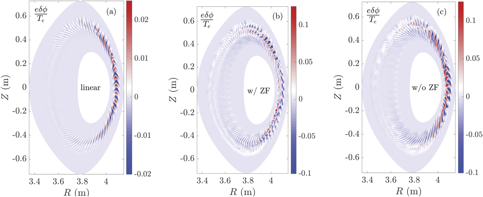
Standard image High-resolution imageFigure 4(a) shows the electrostatic potential in a poloidal cross-section in the simulation with kinetic electrons during the linear phase at time t = 9.6R0/Cs . The eigenmode is localized at the outer mid-plane in the region of low magnetic field strength where the curvature is bad, similar as in tokamaks and it peaks around ψ ∼ 0.26ψw. Figure 4(b) shows the potential at the nonlinear stage at time t = 11.2R0/Cs during the simulation where the zonal flow has been kept (solid blue line in figure 3). In the nonlinear phase where the zonal flow is artificially removed (see figure 4(c)), the linear eigenmode structure starts smearing up due to the nonlinear mode coupling. Whereas, when the zonal flow is included in the simulations, the shear caused by the zonal flow leads to the breaking of these eddies even into finer structures. This behavior was also observed in LHD simulations with adiabatic electrons in a previous GTC work [19]. Figure 5 shows the real space 3D contour plot of the electrostatic potential on the diagnosed flux surface with ψ ∼ 0.28ψw in the linear stage at time t = 9.6R0/Cs (figure 5(a)) and in the nonlinear stage at time t = 11.2R0/Cs (figure 5(b)). Due to k|| ≪ k⊥ property of the microturbulence, the eddies are elongated along the field lines. The flux surface variation of root-mean-squared electrostatic perturbed potential with and without zonal flow, and the radial electric field resulting from the turbulence in the nonlinear stage at time t = 11.2R0/Cs are shown in figure 6. A noticeable difference between the turbulence potential with and without zonal flow can be seen by comparing red and blue lines that indicate the suppression of ITG turbulence due to the zonal flow.

Figure 4. Contour plots of the electrostatic perturbed potential in the linear phase at t = 9.6R0/Cs (a), in the nonlinear phase at t = 11.2R0/Cs with zonal flow (b) and in the nonlinear phase without zonal flow (c), of ITG turbulence simulation with kinetic electrons on a poloidal plane.
Download figure:
Standard image High-resolution image
Figure 5. The real space 3D contour plots of the electrostatic potential on the diagnosed flux surface with ψ = 0.28ψw in the linear phase at time t = 9.6R0/Cs (a) and in the nonlinear phase at time t = 11.2R0/Cs with zonal flow (b).
Download figure:
Standard image High-resolution image
Figure 6. The flux surface variation of the root-mean-squared electrostatic perturbed potential (δϕRMS) with (red line) and without (blue line) zonal flow and the radial electric field (Er
) (black line) resulting from the turbulence during the nonlinear stage of ITG turbulence simulations at time t = 11.2R0/Cs
. The electrostatic potential is normalized with Te/e, and the radial electric field resulting from the turbulence is normalized with  .
.
Download figure:
Standard image High-resolution imageFigure 7 shows the toroidal spectrum, for m = n/ι, in the linear (blue) and nonlinear (red) phase of the simulation with kinetic electrons with zonal flow. The spectrum in the linear phase is narrow in the toroidal mode number with a maximum at n = 50 and an approximate width of Δn ∼ 20. Linear simulations (not shown here) indicate that the most dominant eigenmode is n = 50, m = 100 with a frequency of ω = 4.10Cs /R0, propagates in the ion diamagnetic drift direction and has a growth rate of γ = 1.47Cs /R0 which is approximately 1.5 times larger than in adiabatic electron simulations (γ = 0.96Cs /R0 and ω = 3.40Cs /R0). As there is no resonant interaction of the trapped electrons with the ITG modes, the response of trapped electrons to the ITG turbulence is almost zero, rather than adiabatic. Therefore, the dielectric constant in the gyrokinetic Poisson equation decreases when the trapped electron population increases. This provides a mechanism for increasing the ITG growth rate. The normalized perpendicular wavenumber corresponding to the dominant mode is k⊥ ρi = 1.1. In the nonlinear phase, the toroidal spectrum in figure 7 (averaged over time from 14.4R0/Cs to 17.6R0/Cs ), after an inverse cascade [19], becomes broader due to the nonlinear mode coupling.

Figure 7. The comparison of toroidal mode spectrum along m = n/ι in the linear and nonlinear phase of the ITG turbulence simulation using kinetic electrons.
Download figure:
Standard image High-resolution image3.2. TEM
Trapped electron mode (TEM) driven turbulence is another dominant channel for transport in fusion plasmas which is destabilized due to the presence of density and/or electron temperature gradient. TEM turbulence simulations are mostly performed in LHD with flux-tube code GKV [16, 17] where the effects of isotopes and collisions on microinstabilities and the role of zonal flow on TEM turbulence in LHD have been studied, as discussed in section 1. In this section, the global nonlinear pure TEM turbulence simulations have been carried out using GTC.
The plasma profile used for the simulations is illustrated in figure 8. The maximum normalized density gradient is R0/Ln
∼ 47.2, where  , and also peaks at ψ ∼ 0.33ψw. Temperature profiles are homogeneous along the plasma, Ti = Te = 1 keV, so η = 0. The simulation domain, represented by dashed black lines, is kept the same as in section 3.1. Based on the convergence studies, mesh and number of particles are the same as described in section 3.1 but the time step used is 0.016Cs
/R0.
, and also peaks at ψ ∼ 0.33ψw. Temperature profiles are homogeneous along the plasma, Ti = Te = 1 keV, so η = 0. The simulation domain, represented by dashed black lines, is kept the same as in section 3.1. Based on the convergence studies, mesh and number of particles are the same as described in section 3.1 but the time step used is 0.016Cs
/R0.

Figure 8. Radial profiles for the equilibrium ion temperature Ti and electron temperature Te (blue dashed line), the ion and electron density profile (blue solid line), the normalized density gradient R0/Ln (red solid line), used for the simulations of TEM turbulence with η = 0. The black dashed lines represent the simulation boundary with ψinner = 0.08ψw and ψouter = 0.7ψw.
Download figure:
Standard image High-resolution imageFigure 9 shows the time history of two TEM simulations: one where the self-generated zonal flow has been kept (solid lines) and another where the zonal flow has been removed (dashed lines). The three quantities represented are the ion diffusivity averaged over ψ ∈ [0.19, 0.45]ψw normalized by the gyro-Bohm value (red lines), radial electric field resulting from the turbulence (black line) and the root-mean-squared perturbed electrostatic potential (blue lines). It has been confirmed that De ∼ Di. First, turbulent transport exponentially grows during the linear phase, and then, due to mode coupling, inverse cascade from high to low mode number, and zonal flow interaction, it finally saturates. However, the zonal flow is not acting as the dominant saturation mechanism as can be seen from the simulations with and without zonal flow. In other words, the zonal flow in TEM simulations is not as important as it was for ITG saturation. The role of zonal flow in TEM turbulence suppression has been widely discussed for axisymmetric tokamaks [30–37] and it is shown that the role of zonal flow is usually weak in TEM turbulence regulation. Although the TEM turbulence regulation by zonal flow depends upon the parameters such as magnetic shear, electron to ion temperature ratio, electron temperature gradient and ηe [33–35]. Additionally, the conclusions drawn for tokamak may or may not be consistent for LHD as the neoclassical radial electric field may have a considerable effect on the turbulent transport in stellarators [18, 51]. It could be a future study to explore this complex parameter landscape.

Figure 9. Time history of the ion diffusivity averaged over ψ ∈ [0.19, 0.45]ψw (red) and non-zonal electrostatic perturbed potential (blue) with zonal flow (solid) and without zonal flow (dashed) and zonal electric field (black). The diffusivity is normalized by the gyro-Bohm diffusivity and the electrostatic potential is normalized by Te/e, the radial electric field resulting from the turbulence is normalized with  .
.
Download figure:
Standard image High-resolution imageFigure 10(a) shows the electrostatic potential on a poloidal plane during the linear phase at time t = 3.2R0/Cs , TEM eigenmode shows a thinner mode structure than ITG simulations. Like ITG turbulence, TEM turbulence is extended along the magnetic field lines and localized in the region of low magnetic field strength where the normal curvature is unfavorable and peaks at ψ ∼ 0.30ψw. Figures 10(b) and (c) shows the potential during the nonlinear phase at time t = 6.4R0/Cs for a simulation with and without zonal flows respectively. Turbulence spreading is observed during the nonlinear phase but the turbulent eddies are barely affected by zonal flows. Unlike ITG turbulence, the zonal flow is not playing an important role in the case of TEM turbulence. That is consistent with figure 9 where we previously discussed the little differences of the simulations with and without zonal flow. Figure 11(a) shows the contour plot of the electrostatic potential on the diagnosed flux surface ψ ∼ 0.28ψw in the 3D real space during the linear phase at time t = 3.2R0/Cs . Like ITG turbulence, the eddies are elongated along the field lines. Figure 11(b) shows the contour plot of electrostatic potential in 3D real space in the nonlinear stage at time t = 6.4R0/Cs , with zonal flow. Figure 12 shows the flux surface variation of root-mean-squared electrostatic perturbed potential with and without zonal flow, and the radial electric field resulting from the turbulence. The red and blue lines are almost overlapping with each other, re-affirming that the zonal flow is not playing an important role in the TEM turbulent transport.

Figure 10. Contour plots of the electrostatic perturbed potential in the linear phase at t = 3.2R0/Cs (a), in the nonlinear phase at t = 6.4R0/Cs with zonal flow (b) and in the nonlinear phase without zonal flow (c), of TEM turbulence simulation with kinetic electrons on a poloidal plane.
Download figure:
Standard image High-resolution image
Figure 11. The real space 3D contour plots of the electrostatic potential on the diagnosed flux surface with ψ = 0.28ψw in the linear phase at time t = 3.2R0/Cs (a), and in the nonlinear phase with zonal flow at time t = 6.4R0/Cs (b).
Download figure:
Standard image High-resolution image
Figure 12. The flux surface variation of the root-mean-squared electrostatic perturbed potential (δϕRMS) with (red line) and without (blue line) zonal flow and the radial electric field (Er
) (black line) resulting from the turbulence during the nonlinear stage of TEM turbulence simulations at time t = 6.4R0/Cs
. The electrostatic potential is normalized with Te/e, and the radial electric field resulting from the turbulence is normalized with  .
.
Download figure:
Standard image High-resolution imageThe toroidal mode spectrum, for m = n/ι, at the linear (blue line) and nonlinear (red line) phases during a nonlinear TEM simulation is represented in figure 13. The linear spectrum indicates that the dominant eigenmode is n = 140, m = 280 with a linear growth rate γ = 3.96Cs /R0, frequency ω = 0.55Cs /R0 and normalized perpendicular wavenumber k⊥ ρi = 2.7. The ratio |ω/γ| < 1 implies that this TEM simulation may be reactive turbulence [52]. During the nonlinear saturation (averaged over time from 6.4R0/Cs to 9.6R0/Cs ), the nonlinear poloidal and toroidal mode coupling leads to an inverse cascade from high to low mode numbers [53].

Figure 13. The comparison of toroidal mode spectrum along m = n/ι in the linear and nonlinear phase of the TEM turbulence simulation.
Download figure:
Standard image High-resolution imageWe have carried out further TEM simulations with different normalized density gradients R0/Ln
. Figure 14 shows the variation of the linear growth rate and frequency of the dominant TEM turbulent mode for each simulation. The linear instability threshold for the TEM turbulence is found for values of the normalized density gradient around  . The growth rate increases almost linearly with the gradient although the frequency barely increases. As the gradient increases the spectrum also shifts to higher toroidal mode numbers. The nonlinear physics of the TEM turbulent transport show similar features as has been previously discussed in this section.

Figure 14. The variation of the real frequency and growth rate of the most dominant TEM mode with the normalized density gradient R0/Ln .
Download figure:
Standard image High-resolution image3.3. Turbulence for η = 1 case
In the previous sections, the microturbulences studied are pure ITG and pure TEM in which either the ion temperature gradient or density gradient is present. But in general, both the temperature and density gradients are present in an experiment [16, 17]. In this section, an additional case is studied by taking into account the gradient in both the ion temperature and the plasma density while keeping the electron temperature profile uniform, and a comparison of the nonlinear turbulent transport for the cases with η = 0, 1, and ∞ is made. Figures 2 and 8 show the profiles used for the cases with η = ∞ and η = 0 that are discussed in sections 3.1 and 3.2 corresponding to the ITG and TEM turbulence respectively. For η = 1 case, the maximum of normalized ion temperature and density gradients are  and R0/Ln
∼ 47.2. The shape of the plasma profile is the same as is used for the cases with η = ∞ and 0. The maximum of gradients in profile is present at ψ ∼ 0.33ψw. The on-axis ion and electron temperature are 2 keV and 1 keV respectively. Based on the convergence studies, simulation parameters and mesh are the same as described in section 3.2.
and R0/Ln
∼ 47.2. The shape of the plasma profile is the same as is used for the cases with η = ∞ and 0. The maximum of gradients in profile is present at ψ ∼ 0.33ψw. The on-axis ion and electron temperature are 2 keV and 1 keV respectively. Based on the convergence studies, simulation parameters and mesh are the same as described in section 3.2.
The linear spectrum shows that the dominant mode is n = 160, m = 325 with the growth rate γ = 3.72Cs /R0, frequency ω = 4.74Cs /R0 and normalized perpendicular wavenumber k⊥ ρi = 3.5, propagating in the ion diamagnetic drift direction. So, the simulation is dominated by ITG turbulence. The electrostatic potential looks like the typical ITG mode structure localized on the outer mid-plane side. In the nonlinear phase, the zonal flow regulates the turbulent transport by reducing it by almost two times. The comparison of the turbulent transport levels for the three cases is shown in figure 15. The ion transport coefficients (χi, Di) are averaged over ψ ∈ [0.19, 0.45]ψw. It has been confirmed that De ∼ Di. The zonal flow physics has been included in all three cases. For η = 1, two distinct saturations have been observed. The first saturation happens at t ∼ 3.7R0/Cs and the second saturation happens at t ∼ 5.0R0/Cs . Unlike the cases η = ∞ and η = 0, the spectrum for the η = 1 case is quite broad, comprising low and high numerical modes. The high numerical modes saturate first in the nonlinear phase while the low numerical modes saturate later which leads to two distinct saturations. The volume averaged ion diffusivity and conductivity are almost the same for the η = 1 case. The transport with η = ∞ case is the highest, while η = 0 has the lowest transport level. From this comparison, it is concluded that in the present scenario for similar plasma profile gradients, the ITG turbulence acts as the primary drive for the heat conductivity transport, whereas the TEM turbulence is effective for the particle diffusivity.

Figure 15. The time history comparison of the transport averaged over ψ ∈ [0.19, 0.45]ψw for η = 0, 1, and ∞.
Download figure:
Standard image High-resolution image
4. Conclusion and discussion
In this work, we have presented global gyrokinetic simulations of transport induced by microturbulence arising from the pure ITG and pure TEM instabilities in the LHD stellarator. The pure ITG turbulence is excited by the gradient in ion temperature while keeping the other profiles uniform. The effect of kinetic electrons on the ITG turbulence is studied using the hybrid model which is well-benchmarked in GTC. The kinetic electrons increase the linear growth rate of the ITG turbulence by  times and the turbulent transport by
  times as compared to the case with adiabatic electrons. The pure TEM turbulence is excited by the density gradient in the plasma species. The eigenmode structure in the linear phase for the TEM turbulence is localized on the outer mid-plane side where the curvature is bad, similar to that in tokamaks and ITG turbulence. The TEM linear mode structure is thinner and radially localized as compared to the ITG linear eigenmode. The nonlinear simulations of TEM turbulence with and without zonal flow show that, unlike in ITG turbulence, zonal flow is not playing an important role in regulating the transport by TEM turbulence. In tokamaks, the regulation of TEM turbulence by zonal flow is weak although different works by independent codes have shown significant effect of zonal flow when some parameters are changed such as magnetic shear, electron to ion temperature ratio, electron temperature gradient and ηe [33–35]. For example, the lower magnetic shear has negligible effect on transport due to TEM turbulence. However, at larger magnetic shear, the radial streamer is easier to be broken by zonal flow due to turbulence elongation in the radial direction [33]. For cold ions and steeper electron temperature gradient, shear caused by zonal flow is weak in tokamaks [34] and also with the realistic plasma profiles, for ηe > 1, zonal flow effect is weak [35]. It could be a future study to explore this complex parameter space for the effect of zonal flow on TEM turbulence in LHD. Further, the comparison between different cases with η = 0, 1, and ∞ in LHD shows that the turbulent transport levels in the nonlinear saturation is highest for η = ∞ case and lowest for η = 0 case. Thus, in the present scenario for similar plasma profile gradients, the ITG turbulence acts as the primary drive for the heat conductivity transport whereas the TEM turbulence is effective for the particle diffusivity.
Acknowledgment
The authors would like to thank J. Riemann, R. Kleiber, and D.A. Spong for providing the equilibrium data of the LHD. We acknowledge technical support by the GTC team. This work is supported by the Board of Research in Nuclear Sciences (Sanctioned No. 39/14/05/2018-BRNS), Science and Engineering Research Board EMEQ program (Sanctioned No. EEQ/2017/0001-64), National Supercomputing Mission (Ref No.: DST/NSM/R&D_HPC_Applications/2021/4) and Infosys Young Investigator award. A.S. is thankful to the Indian National Science Academy (INSA) for their support under the INSA Honorary Scientist Fellowship scheme. This work was partially supported by the US Department of Energy, under Award No. DE-SC0018270 (SciDAC ISEP Center), DE-FG02-07ER54916, DE-SC0020413. The results presented in this work have been simulated on ANTYA cluster at Institute of Plasma Research, Gujarat, India, and SahasraT supercomputer at Indian Institute of Science, Bangalore, India, and the US National Energy Research Scientific Computing Center (DOE Contract No. DE-AC02-05CH11231).