
Abstract
Objective. The current practices of designing neural networks rely heavily on subjective judgment and heuristic steps, often dictated by the level of expertise possessed by architecture designers. To alleviate these challenges and streamline the design process, we propose an automatic method, a novel approach to enhance the optimization of neural network architectures for processing intracranial electroencephalogram (iEEG) data. Approach. We present a genetic algorithm, which optimizes neural network architecture and signal pre-processing parameters for iEEG classification. Main results. Our method improved the macro F1 score of the state-of-the-art model in two independent datasets, from St. Anne's University Hospital (Brno, Czech Republic) and Mayo Clinic (Rochester, MN, USA), from 0.9076 to 0.9673 and from 0.9222 to 0.9400 respectively. Significance. By incorporating principles of evolutionary optimization, our approach reduces the reliance on human intuition and empirical guesswork in architecture design, thus promoting more efficient and effective neural network models. The proposed method achieved significantly improved results when compared to the state-of-the-art benchmark model (McNemar's test, p ≪ 0.01). The results indicate that neural network architectures designed through machine-based optimization outperform those crafted using the subjective heuristic approach of a human expert. Furthermore, we show that well-designed data preprocessing significantly affects the models' performance.
Export citation and abstract BibTeX RIS

Original content from this work may be used under the terms of the Creative Commons Attribution 4.0 license. Any further distribution of this work must maintain attribution to the author(s) and the title of the work, journal citation and DOI.
1. Introduction
Epilepsy is a neurological disorder affecting around 50–60 million people worldwide (Beghi 2020). Epilepsy may be caused by genetic predispositions, developmental disorders, brain injury, stroke, tumor, and others, and is characterized by epileptic recurrent, unprovoked seizures. Anti-seizure medication can eliminate epileptic seizures in about two-thirds of patients. Yet despite a wide array of available medications, about one-third of patients suffer from drug-resistant epilepsy and continue having seizures (Asadi-Pooya et al 2017).
Intracranial electroencephalogram (iEEG) monitoring is one of the key clinical procedures, which selected drug-resistant patients undergo in order to be considered for surgical removal of the epileptogenic zone, the brain area responsible for seizure generation (Rosenow and Lüders 2001). iEEG records electrical signals directly also from deep brain structures and is necessary for precise localization of the pathological epileptic tissue in the brain. The electrodes, which record the brain activity, are implanted predominantly into areas that are suspected to be epileptogenic zones. After the electrode implantation surgery, the patient is monitored for up to four weeks in a VideoEEG monitoring unit. Next, the recorded signals need to be investigated for abnormal activity, such as epileptic discharges, high-frequency oscillations, very-high-frequency oscillations, and especially epileptic seizures, and processed in order to decide about the next step in the treatment.
In current clinical practice, electrophysiologist physicians manually investigate the iEEG recordings to localize epileptic foci. However, this task is very time-consuming and often focused on short segments of pre-ictal (before seizure) and ictal activity. Moreover, it has been shown that the level of agreement in interpretation between experts varies and is biased by the subjective experience of the neurophysiologist (Jing et al 2020). Recently it has been shown that inspection of interictal periods (i.e. periods without epileptic seizures) has valuable diagnostic information for seizure onset zone localization (Cimbalnik et al 2019). Unfortunately, this substantial part of iEEG recordings is frequently omitted during visual inspection of iEEG. In order to overcome these limitations, there has been substantial effort to automatize the iEEG review process.
In a recent study, it has been shown that convolutional neural networks are suitable for this task (Nejedly et al 2019a) achieving remarkable results for the detection of pathological segments and artifacts. However, neural network design can be quite challenging as it is most often based on heuristic rules and previous engineering and deep learning experience. This issue can be overcome by using a genetic algorithm (GA) as an optimization technique for the neural network architecture and feature selection (Wei and Wei 2008, Chang and Yang 2018, Aquino Britez et al 2021).
This work focuses on optimizing neural network architecture hyperparameters and preprocessing that converts the input signal to a usable form for subsequent deep-learning analysis. We experiment with two preprocessing methods i.e. short-time Fourier transform (STFT) and Wavelet transform, which influence the time-frequency representation of our input signal. The model is trained and tested on publicly available datasets from St Anne's University Hospital Brno and Mayo Clinic (Nejedly et al 2020). Subsequently, results are compared with the state-of-the-art CNN-GRU (convolutional-gated recurrent unit) model presented in Nejedly et al (2019b).
2. Methods
2.1. Dataset
For the purposes of this study we used data from a publicly available dataset with iEEG signals (Nejedly et al 2020), which were collected at St. Anne's University Hospital (FNUSA) and Mayo Clinic. The data (sampling frequency 5 kHz) from FNUSA were collected from 30 min of awake interictal resting state from 14 epileptic patients that were undergoing pre-surgical invasive EEG monitoring. The patients were implanted with standard intracranial depth electrodes (ALCIS) and the data were collected with an acquisition system M&I; BrainScope, Czech Republic. The Mayo Clinic data (sampling frequency 5 kHz) comes from 25 patients and was recorded during the first night after electrode implantation (AD-Tech) between 1 am and 3 am. Neuralynx Cheetah system (Neuralynx Inc., Bozeman MT, USA) acquisition system was used for the data collecting and the patients were implanted with either depth electrodes, grids and strips, or a combination of both.
The EEG recordings were manually annotated by three independent reviewers, by using SignalPlant (Plesinger et al 2016, Nejedly et al 2018), a free software tool for signal processing, inspection, and annotation. The annotation is based on visual inspection using power distribution matrices (Brázdil et al 2017). The data are classified based on 4 distinctive events that standardly occur during iEEG measurement, i.e. powerline noise, artifactual signals, physiological activity, and pathological activity. The segments are classified as a physiological activity if there are no artificial signals or epileptic biomarkers. Pathological activity includes segments with epileptiform graphoelements, such as pathological high-frequency oscillations and interictal epileptiform discharges. The number of samples in each class is described in table 1. More information on the dataset can be found in Nejedly et al (2020). Following the annotation, the iEEG data were segmented into 3 s chunks that are fed to the classification model.
Table 1. Overview of data distribution across the classes for the 3 s segments.
| Classification category of iEEG event | Number of samples FNUSA | Number of samples MAYO |
|---|---|---|
| Powerline artefacts | 13 489 | 41 922 |
| Noise artefacts | 32 599 | 41 303 |
| Pathological epileptiform activity | 52 470 | 15 227 |
| Physiological activity | 94 560 | 56 730 |
| Total | 193 118 | 155 182 |
The data segments from FNUSA were randomly split into training (60% of each class) and validation (20% of each class) and testing (20% of each class) data. The validation data were used for model architecture ranking during the optimization process, and the test set was only used to obtain final scores (preventing data overfitting), this process is shown in figure 1. We run the GA on the FNUSA data and use it, as shown in figure 1, for model optimization, development, and result evaluation. Data from Mayo Clinic were used to train the optimized model and report the final results on the test portion of the data. The proposed data split shows that the developed model architecture generalizes to different institutions, which was not used for model development.

Figure 1. Principle of optimization of the neural network with a genetic algorithm with the datasets.
Download figure:
Standard image High-resolution image2.2. Preprocessing
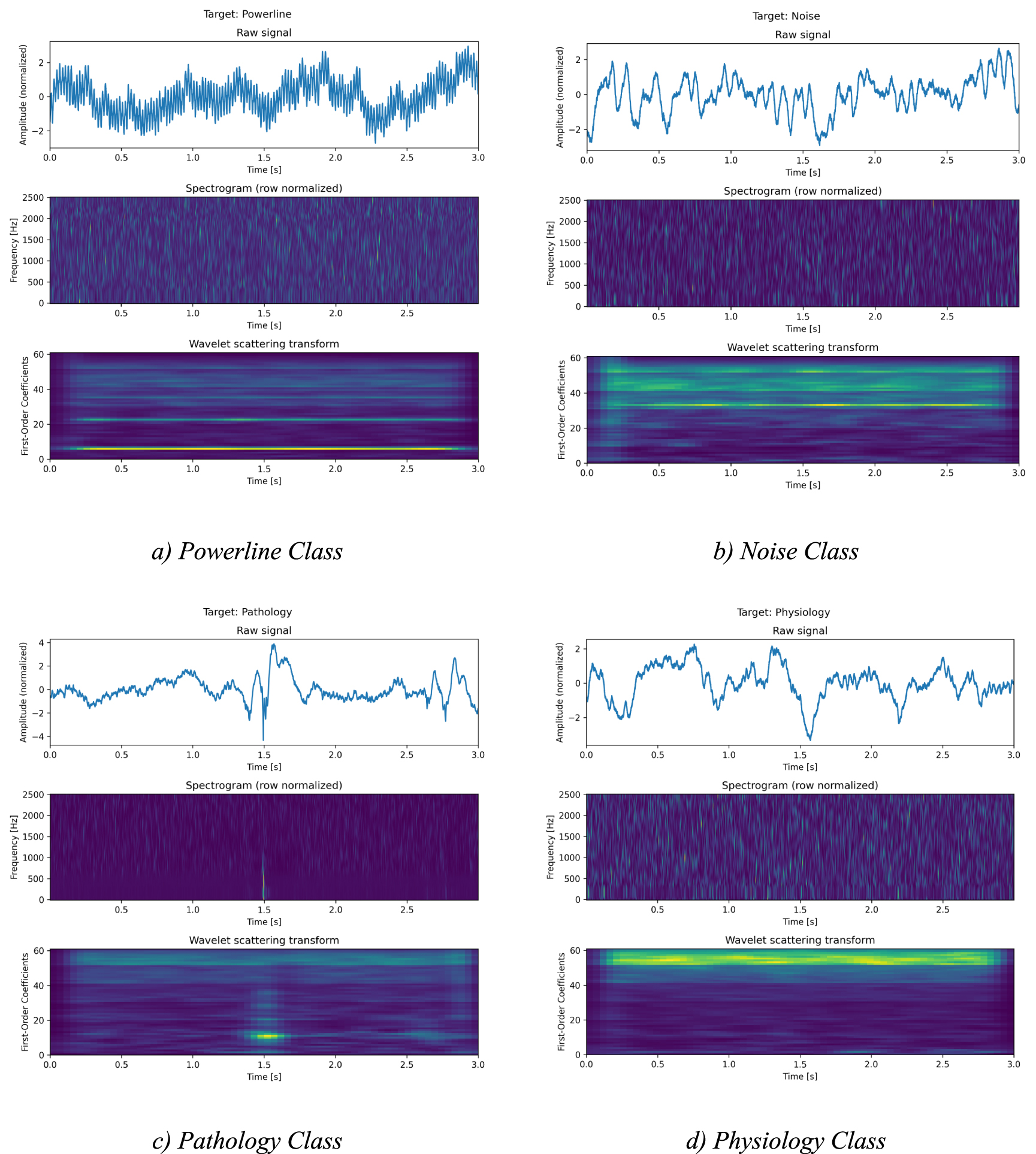
The signal segments (3 s, 15 000 samples) were converted into a time-frequency domain, either by computing the spectrogram by STFT of the signal or by extracting first-order scattering coefficients from a wavelet scattering transform (WST) (Anden and Mallat 2014). The parameters of the STFT and WST were optimized and are shown in table 2. Before the signal representation is passed to the classification model, we normalize it by calculating z-score for each frequency band. Examples of the preprocessing for each of the classes can be seen in figure 2.

Figure 2. Visualization of the preprocessing of the raw signal with the STFT (Hann window, segments per window = 32, overlapping segments = 16, length of zero-padded FFT = 256) and WST (J = 8, Q = 10), where the brighter colors represent higher amplitude and darker colors lower amplitudes of the STFT and WST.
Download figure:
Standard image High-resolution imageTable 2. Overview of optimizable parameters and their nominal value in the benchmark model.
| Encoded parameter | Benchmark model value | GA value range |
|---|---|---|
| Neural network architecture parameters | ||
| Number of filters | 256 | {64, 128, 256, 512, 1024} |
| Kernel size | 3 | {3, 5, 7} |
| Number of hidden nodes | 128 | {64, 128, 256, 512} |
| Number of GRU layers | 1 | {1, 2, 3} |
| Batch size | 64 | {64, 128, 256} |
| Learning rate | 1 × 10⁻³ | {1 × 10⁻³, 5 × 10⁻⁴, 1 × 10⁻⁴} |
| Weight decay | 1 × 10⁻⁴ | {0, 1 × 10⁻⁴, 1 × 10⁻⁶} |
| Spectrogram parameters | ||
| Window function | Tukey | Tukey, Hann, Barlett, Flattop |
| Number of segments (Nperseg) | 256 | {32, 64, 128, 256, 512} |
| Overlapping segments (Noverlap) | 128 | Nperseg // {2, 4, 8, 16, 32, 64} |
| NFFT | 1024 | {32, 64, 128, 256, 512, 1024} |
| WST parameters | ||
| J | — | {3, 4, 5, 6, 7, 8, 9, 10} |
| Q | — | {2, 3, 4, 5, 6, 7, 8, 9, 10} |
Example of the encoded genome with direct encoding: Hann window, with 32 segments and 16 overlapping segments and padded FFT of length 128, convolutional layer with 256 filters, kernel size of 3, GRU layer with 3 layers and 512 hidden nodes, batch size of 64, learning rate 5 × 10⁻⁴ and weight decay 0 would be represented as [1, 5, 2, 7, 8, 3, 9, 2, 6, 0.0005, 0].
For the spectrogram computation, we use SciPy library (Virtanen et al 2020), where the window type, length of each segment, number of overlapping segments, and length of zero-padded fast Fourier transform (FFT) are parameters that we want to optimize. The computation of the WST, from which we extract the first-order coefficients as our model input, is done through Kymatio library (Andreux et al 2020, 1–6). The coefficients can be changed by varying parameters J and Q, which specify an average scale as a power of two and the number of wavelets per octave respectively.
2.3. Neural network architecture optimization methods
In general, neural network hyperparameters can be optimized using various methods such as random search, grid search, Bayesian optimization, particle swarm optimization, and GAs (Yu and Zhu 2020). Recently, researchers developed techniques to optimize topologies of neural network architectures based on various strategies such as reinforcement learning, GAs, or neuroevolution (Zoph and Le 2016, Aszemi and Dominic 2019, Stanley et al 2019).
In order to evaluate all combinations of hyperparameters inspected in this paper we estimated that 180 years of computing would be required. For this reason, we designed a custom method for hyperparameter optimization based on a GA, which allows asynchronous computing using multiple GPUs. The main motivation for using the GA framework method is that we plan to expand the method to allow topology optimization in the future. At the same time, we designed the method in a way that optimization variables can be composed of continuous, discrete, binary, and nominal data.
2.4. GAs
GA, inspired by Darwin's evolution theory, is an optimization technique utilizing population-based metaheuristic search algorithm, based on the survival of individuals with the fittest genes in the population. The general principle of the GA is based on a selection of the fittest candidates, that either pass their genes onto their offspring or appear again in the new generation, and thus converge to an optimal solution.
In general, there are two approaches to problem-solving on which the effectiveness of the algorithm relies, namely exploration and exploitation. In the exploration phase, the algorithm actively searches for new solutions, while the exploitation phase is more focused on a refinement of already existing solutions so that the fitness score will quickly improve. Should the exploration be too strong, the algorithm might resemble a random search and would take a long time to convert. In the other case, where exploitation would strongly dominate without properly covering the search space, the algorithm might convert to a local minimum. The trade-off between both cases is usually adaptively updated during the optimization process.
In this study, we use a custom asynchronous GA, illustrated in figure 3 that uses the fittest candidates to optimize the neural network architecture (described in the next section) used for iEEG processing. The algorithm was mainly developed in order to allow asynchronous evaluation, which significantly speeds the optimization process by utilizing multiple GPUs for model asynchronous training. We measure the fitness of each neural network architecture with a kappa score, reflecting the model's classification performance compared with the expert gold standard while accounting for random chance.

Figure 3. Principle of asynchronous GA distribution across multiple GPUs, where the genome encoding of the individuals is represented with general parameters P.
Download figure:
Standard image High-resolution imageThe candidates that will become parents are chosen with a tournament selection, by being the most fit within a group of three randomly selected individuals from the generation. This way, the fitter candidates have a higher chance to become parents, but the less fit individuals are not excluded completely, which is important for diversity during the exploration phase. The individuals that won the tournament selection then become parents by forming pairs with others. This way they pass a combination of their genes onto an offspring, which will compete in the next generation. For this, we use a uniform crossover (Umbarkar and Sheth 2015), which combines randomly sampled genes of both parents and creates two offspring. The genes the offspring inherits from parent A are randomly sampled and filled in by complementary genes from parent B, as can be seen in the crossover part in figure 4. The second offspring inherits genes from A and B that the first offspring did not inherit, creating thus a second unique genome. Moreover, there is also a small probability that one or more genes of the new offspring will be changed for another random valid value during a mutation. Should a genotype that was already evaluated in earlier generations appear, it is removed from the new generation and the algorithm gets a chance to replace it with a randomly generated genotype. This process is illustrated in figure 4.

Figure 4. Schematic demonstration of the process of creating new offspring with the genetic algorithm, where the genome encoding of the individuals is represented with general parameters P.
Download figure:
Standard image High-resolution imageIn this study, we optimize parameters that can be classified into two groups. The first group consists of hyperparameters of our classification model and includes the size of a convolutional kernel, the number of convolutional filters, the number of hidden nodes in GRU layers, the number of GRU layers, batch size, learning rate, and weight decay. The second group of hyperparameters optimizes iEEG signal preprocessing, either STFT hyperparameters (window type, segment length, number of overlapping segments, and size of zero padding FFT) or WST parameters J (maximum log-scale of the scattering transform) and Q (number of wavelets per octave for the first order). The overview of the parameters can be found in table 2.
2.5. Deep learning model architecture
The parameter optimization in this work was done on a CNN-GRU architecture presented in a study from Nejedly et al (2019b). While the results achieved in the original study were remarkable, the model was designed empirically. Thus in this following study, we aim on improving the model performance, by automatically optimizing the parameters of the given model. The model was implemented with a Pytorch library (Paszke et al 2017) while trained and optimized on a GPU server with 2× Intel(R) Xeon(R) Gold 6248R CPU@3.00 GHz with 1.41 TB RAM memory and up to 8 available NVIDIA Quadro RTX 5000 GPUs.
The model itself was designed to classify different iEEG events based on a spectrogram input. The architecture of the model consists of a convolutional layer with a ReLU activation function that extracts spatial features from the spectrogram. The output of the convolutional layer is normalized with a batch normalization layer and after reshaping is passed into a GRU layer, followed by a fully connected layer with a Softmax activation function. During the training, the model uses an Adam optimizer and cross-entropy loss. The architecture of the model, with the highlighted features, that are considered for optimization can be seen in figure 5.

Figure 5. CNN-GRU model with highlighted optimizable parameters in blue.
Download figure:
Standard image High-resolution image2.6. Optimization
In order to evaluate all combinations of the parameters for the STFT-Model and WST-Model with an average training time of 30 min, we would need approximately 180 years of computing per one GPU. Optimization algorithms, such as grid search or random search thus would not be much effective. We thus decided to split the optimization process into two parts, exploration and exploitation-focused GA, which converges to an optimal solution much faster. This algorithm allows us to distribute the optimization over multiple GPUs, which enables further speeding of the optimization process. We got the final solution after two days of computing on the multiple GPUs, which corresponds to about ten days of computing time when using a single GPU only.
During the exploration, the GA searched for solutions from different parts of the search space. The algorithm was set up to evolve up to 30 generations, where each generation consisted of 20 individuals. Each new generation consisted of 20% of new, randomly generated genotypes, and the 80% of the individuals were created from the previous generation by crossover operation and a mutation with a rate of 0.1. To limit the search space, we also observed the influence of the model hyperparameters while keeping the preprocessing hyperparameters constant, and secondly optimizing signal preprocessing parameters while keeping the model architecture constant.
After the exploration phase, we had around 1000 solutions available and joined the search of both parameter groups to continue the search for the optimal solution. As the training became more computationally expensive and took a longer time, we distributed the training over six GPUs, which required adjustments in implementing the GA, illustrated in figure 3. In this asynchronous parallel implementation, we created a server that guides the optimization process and automatically assigns optimization tasks to available workers (docker images each with a single GPU).
The initial population of size 20 was randomly initialized by solutions from the exploration part. Additionally, combinations of three of the best solutions for the model hyperparameters and two of the best signal-processing parameters were included in the initial population. This way, we utilized the search from the exploration part and helped the model speed up the search, while still allowing it to explore the search space. Once all of the initial genotypes have been evaluated, new ones are created when a GPU is available for the computation. The new individuals are created based on the tournament selection and parent breeding described above. To support faster convergence of the algorithm, we include elitism by adding 3, so far, best-performing individuals to the pool of tournament candidates and decrease the mutation rate to 0.05. The parameter search stops when a convergence criterion is met, or when 150 iterations were evaluated.
2.7. Evaluation metrics
In this study, we monitor four metrics, kappa score, F1 score, an area under the receiver operating characteristic (AUROC), and an area under the precision-recall curve (AUPRC). All of those metrics can be used when working with imbalanced data and were also used in previous studies on this dataset, see Nejedly et al (2019b).
We decided to use the kappa score as a fitness function to evaluate the solutions found by the GA. The interpretability of Cohen's kappa is more intuitive than that of the F1. Compared to a macro F1, Cohen's kappa is a more strict metric as it also considers a probability of random agreement in the final score.
The kappa metric is used to measure how closely the classified instances match the ground truth labels while controlling the accuracy of a random classifier (Cohen 1960). The interpretation of Cohen's kappa (McHugh 2012) is summarized in table 3 with a described level of agreement between the raters and the responding percentage of data accuracy. The general kappa score can be computed as follows:
Table 3. Kappa interpretation.
| Value of kappa | Level of agreement |
|---|---|
| 0–0.20 | None to slight |
| 0.21–0.39 | Minimal |
| 0.40–0.59 | Weak |
| 0.60–0.79 | Moderate |
| 0.80–0.90 | Strong |
| >0.90 | Almost perfect to perfect |

3. Results
Tables 4 and 5 offer an overview of five best solutions found by the GA for each the STFT and the WST models and the convergence of the algorithm in the exploitation phase is shown in figures 6(a) and (b). The chosen parameters of the STFT-Model and the WST-Model used for reporting the final results are highlighted in tables 4 and 5.

Figure 6. Convergence of the STFT (a) and WST (b) models during the asynchronous optimization (exploitation part).
Download figure:
Standard image High-resolution imageTable 4. Overview of top five solutions for the STFT model parameter search.
| Window | NPerseg | Overlap | NFFT | Conv filters | Conv kernel | Hidden nodes | GRU layers | Batch size | LR | L2 | Kappa score |
|---|---|---|---|---|---|---|---|---|---|---|---|
| Hann | 32 | 16 | 128 | 256 | 3 | 512 | 2 | 64 | 5 × 10⁻⁴ | 0 | 0.8885 |
| Hann | 32 | 16 | 256 | 256 | 5 | 512 | 3 | 32 | 5 × 10⁻⁴ | 0 | 0.8875 |
| Hann | 32 | 16 | 256 | 32 | 3 | 512 | 2 | 16 | 5 × 10⁻⁴ | 0 | 0.8870 |
| Hann | 64 | 16 | 128 | 256 | 3 | 512 | 2 | 32 | 5 × 10⁻⁴ | 0 | 0.8863 |
| Hann | 32 | 16 | 256 | 256 | 5 | 512 | 2 | 128 | 5 × 10⁻⁴ | 0 | 0.8849 |
Abbreviations for the table: STFT parameters: Window—type of window function, NPerseg—length of each segment, Overlap—number of overlapping points between segments, NFFT—length of used FFT with zero padding. Model parameters: Convolutional filters—number of output filters for next layer, Convolutional kernel—size of convolving kernel, GRU hidden nodes—number of features in hidden state of a GRU layer, GRU layers—number of recurrent layers, Batch size—number of samples propagated through the network at a time, LR—learning rate, L2—weight decay.
Table 5. Overview of top five solutions for the WST model parameter search.
| J | Q | Conv filters | Conv kernel | Hidden nodes | GRU layers | Batch | LR | L2 | Kappa score |
|---|---|---|---|---|---|---|---|---|---|
| 8 | 10 | 256 | 5 | 512 | 2 | 128 | 1 × 10⁻³ | 0 | 0.9295 |
| 8 | 10 | 512 | 7 | 128 | 3 | 64 | 1 × 10⁻³ | 0 | 0.9294 |
| 7 | 10 | 512 | 5 | 512 | 2 | 128 | 5 × 10⁻⁴ | 1 × 10⁻⁵ | 0.9293 |
| 7 | 10 | 1024 | 3 | 256 | 3 | 128 | 1 × 10⁻³ | 1 × 10⁻⁵ | 0.9292 |
| 7 | 10 | 1024 | 7 | 256 | 3 | 128 | 1 × 10⁻³ | 1 × 10⁻⁵ | 0.9291 |
Abbreviations for the table: WST parameters: J—maximum log-scale of the scattering transform, Q—number of wavelets per octave for the first order. Model parameters: Convolutional filters—number of output filters for next layer, Convolutional kernel—size of convolving kernel, GRU hidden nodes—number of features in hidden state of a GRU layer, GRU layers—number of recurrent layers, Batch size—number of samples propagated through the network at a time, LR—learning rate, L2—weight decay.
An overview of final results is reported in table 6, where the results are averaged over five runs on the test datasets for FNUSA and MAYO. We compare the results on the benchmark model and on the best-found solution for the STFT-Model and the WST-Model parameters. We can observe an increase in all measured metrics scores after the optimization process. Table 7 provides better insight into the impact of the improved performance on the classes, monitoring the F1 score, AUROC, and AUPRC for each class.
Table 6. Comparison of the overall performance between the benchmark model and the best STFT and WST models.
| Kappa score | Macro F1 | Mean AUROC | Mean AUPRC | |
|---|---|---|---|---|
| FNUSA Dataset | ||||
| Benchmark Model | 0.8450 | 0.9076 | 0.9823 | 0.9613 |
| GA STFT-Model | 0.9079 | 0.9419 | 0.9922 | 0.9837 |
| GA WST-Model | 0.9411 | 0.9673 | 0.9969 | 0.9938 |
| MAYO Dataset | ||||
| Benchmark Model | 0.8885 | 0.9222 | 0.9897 | 0.9740 |
| GA STFT-Model | 0.9011 | 0.9344 | 0.9919 | 0.9805 |
| GA WST-Model | 0.9123 | 0.9400 | 0.9941 | 0.9856 |
Table 7. Detailed results of F1 score, AUROC, and AUPRC for each of the classification categories compared between the benchmark model and the best STFT and WST models.
| F1 score | AUROC | AUPRC | |||||||
|---|---|---|---|---|---|---|---|---|---|
| BM | STFT | WST | BM | STFT | WST | BM | STFT | WST | |
| FNUSA Dataset | |||||||||
| Powerline | 0.9934 | 1.0 | 1.0 | 0.9999 | 1.0 | 1.0 | 0.9994 | 1.0 | 1.0 |
| Noise | 0.8152 | 0.8780 | 0.9475 | 0.9687 | 0.9873 | 0.9886 | 0.8962 | 0.9529 | 0.9886 |
| Pathology | 0.8829 | 0.9217 | 0.9451 | 0.9763 | 0.9880 | 0.9984 | 0.9509 | 0.9763 | 0.9881 |
| Physiology | 0.9054 | 0.9311 | 0.9593 | 0.9675 | 0.9817 | 0.9847 | 0.9624 | 0.9792 | 0.9925 |
| MAYO Dataset | |||||||||
| Powerline | 0.9898 | 0.9953 | 0.9970 | 0.9995 | 0.9999 | 0.9999 | 0.9992 | 0.9999 | 0.9999 |
| Noise | 0.8779 | 0.8841 | 0.9042 | 0.9822 | 0.9844 | 0.9899 | 0.9529 | 0.9577 | 0.9740 |
| Pathology | 0.9232 | 0.9512 | 0.9499 | 0.9963 | 0.9984 | 0.9984 | 0.9751 | 0.9881 | 0.9893 |
| Physiology | 0.9013 | 0.9051 | 0.9216 | 0.9807 | 0.9847 | 0.9892 | 0.9690 | 0.9754 | 0.9818 |
McNemar's test based on these results of the benchmark and the optimized WST model shows that for both datasets (table 8), the optimized model significantly improved the final accuracy with a p-value ≪ 0.01.
Table 8. Contingency tables for McNemar's test on FNUSA (a) and MAYO (b) datasets with resulting p-values ≪ 0.01.
| (a) | ||
| FNUSA | BM Correct | BM False |
| WST Correct | 33 917 | 3214 |
| WST False | 626 | 867 |
| (b) | ||
| MAYO | BM Correct | BM False |
| WST Correct | 27 797 | 1545 |
| WST False | 893 | 801 |
4. Discussion
This study is focused on developing GA for hyperparameter optimization of neural networks used for processing of iEEG signals. We identified a set of model and preprocessing hyperparameters that might have the potential to improve the method. Our analysis suggested that with an average training time of 30 min, we would need approximately 180 years of computing per one GPU to verify all possible combinations. The implemented GA with distributed computation over multiple GPUs was able to converge to improved solution within two days (ten days if computed on single GPU). For this reason, we introduce a hyperparameter optimization technique based on a GA, which improves the performance of the state-of-the-art method by optimizing the parameters of the neural network and signal preprocessing. To further decrease computational time needed for convergence, we designed the method allowing for asynchronous evaluation utilizing multiple GPUs.
Results in table 6 show improvement of all observed metrics for both optimized models (STFT and WST). The model with WST showed better results than the model with STFT signal preprocessing. The WST-Model trained on the FNUSA dataset improved the mean AUROC score of 0.9823 and mean AUPRC score of 0.9613 to 0.9969 and 0.9938 respectively, compared to the benchmark CNN-GRU model. The final kappa score of 0.9411 and macro F1 score of 0.9673 showed improvement as well compared to the benchmark model by 0.1 and 0.06 respectively.
Moreover, the final results improved not only on the FNUSA dataset, which was used for the parameter optimization but also on the model re-trained on Mayo Clinic data. The improvement of the separate classes can be seen in more detail in table 7. The increment of the final score is caused mainly by improved classification of noise and physiology classes and, most importantly, also of the pathology class, whose F1 score improved from 0.8829 to 0.9451.
Examples of the output probabilities of the benchmark model and the WST-model are shown in figure 7. Figure 7(a) shows, that the WST-model definitely recognized the pathology class based on the spike occurring at 1.4 s and kept the output probability constant, whilst the benchmark model actually decreased its confidence in the pathology class after the occurring spike and decided in the end for a physiology class. In figure 7(b) we can see that the probabilities of the optimized WST-model are also more smooth compared to the spiky benchmark output probabilities. This effect is most probably caused by better information distillation and less noise in the found classification pattern by the WST-model.

Figure 7. Examples of the output probabilities from the neural network for all four classes (the decision is made based on the output probabilities at the last timestep).
Download figure:
Standard image High-resolution image
During the exploration part of the optimization search, we observed higher increments in the final score when optimizing the preprocessing of the input signal into the model. At this part, the optimized model hyperparameters increased the kappa score by ∼0.02, whilst the spectrogram and WST parameters caused increments by ∼0.04 and ∼0.06. One of the reasons for this could be the fact that the benchmark model was designed with enough expertise, whilst the choice for the spectrogram parameters in the original was based on visual impression without further fine-tuning.
4.1. Limitations
The GA needed around ten days of computing on a single GPU to find both optimized solutions. While this is a huge improvement over the approximated 180 years that would be needed for a grid search, there is still room to bring the computing time down with methods currently researched in neural architecture search (NAS) (Xie et al 2023). Some of the methods that reduce the computational time that could be transferred to hyperparameter optimization are downscaled dataset methods, learning curve extrapolation, performance predictors, or a parameter- or architecture-level methods that require no training to rank them based on estimated score. These methods would, however, require more thorough research in the field of signal processing, as they are mainly explored with image datasets. Another limitation of this study is that it is merely focused on optimization with the GA. We decided to use the GA based on its success in both hyperparameters optimization for deep learning (DL) (Darwish et al 2020), and its successful applications in NAS (Liu et al 2021). This work can thus be further expanded by designing optimization algorithms that would design the whole architecture of the neural network. The optimized model from this study can be further utilized for applications such as epileptic seizure prediction (Kiral-Kornek et al 2018) or noise detection in iEEG (Nejedly et al 2019a).
4.2. Ethics statement
This study was carried out in accordance with the approval of the Mayo Clinic Institutional Review Board with written informed consent from all subjects. The protocol was approved by the Mayo Clinic Institutional Review Board and St. Anne's University Hospital Research Ethics Committee and the Ethics Committee of Masaryk University. All subjects gave written informed consent in accordance with the Declaration of Helsinki. All methods were performed in accordance with the relevant guidelines and regulations.
5. Conclusion
We present a GA designed for hyperparameters optimization of a neural network utilized for the classification of iEEG recordings from epileptic patients. The optimized parameters significantly improved the score on the St. Anne's University Hospital data, which we used for the optimization and for testing. Furthermore, verification of the found parameters on an external institution on data from the Mayo Clinic showed statistically significant improvement as well. The highest improvement was noticeable mainly in the noise and pathology classes, which can further have a positive effect on pathological activity and noise detection in iEEG.
Acknowledgments
This work was supported by Ministry of Health of the Czech Republic, Project NU22-08-00278; Czech Science Foundation, Project 22-28784S; Supported by Project Nr. LX22NPO5107 (MEYS): Financed by European Union—Next Generation EU; The CAS Project RVO:68081731; European Regional Development Fund—Project ENOCH No. CZ.02.1.01/0.0/0.0/16_019/0000868.
Data availability statement
The data that support the findings of this study are openly available at the following URL/DOI: https://springernature.figshare.com/collections/Multicenter_intracranial_EEG_dataset_for_classification_of_graphoelements_and_artifactual_signals/4681208.