

Abstract
This article presents an interlaboratory comparison (ILC) on Raman spectroscopy as a technique for relative quantification of the two most common polymorphs of titanium dioxide (TiO2)—anatase and rutile—in binary mixtures. Some standard methods are currently employed internationally for the determination of TiO2 content in samples (ISO 591-1, ASTM D3720-90), but require extensive sample preparation, do not distinguish between the two polymorphs or are accurate only for small fractions of either polymorph. Raman spectroscopy is a well-suited characterization technique for measuring and differentiating TiO2 in a fast, non-invasive way, while requiring no particular reagent or sample preparation. Eleven international participants conducted the study under the framework of Versailles Project on Advanced Materials and Standards. The collected data was analyzed by means of partial least squares regression after spectral preprocessing. The resulting models all show discrepancies of lower than 2% from the nominal values in the quantitative analysis over the concentration range of 5%–95% mixture fractions, with many datasets showing substantial improvement margins on this figure. The results of this ILC provide validation of Raman spectroscopy as a reliable method for quantification of TiO2 phases.
Export citation and abstract BibTeX RIS

Original content from this work may be used under the terms of the Creative Commons Attribution 4.0 license. Any further distribution of this work must maintain attribution to the author(s) and the title of the work, journal citation and DOI.
1. Introduction
1.1. Overview
Titanium dioxide (TiO2, also known as titania) is a wide band gap semiconductor of utmost industrial importance, employed for a wide variety of applications, and the most widely employed white pigment in dyes and paints in the world. Because of its bright white color, high index of refraction, chemical stability, high ultraviolet (UV) light absorbance and photocatalytic properties, it has a broad spectrum of applications, ranging from being the most employed white pigment in dyestuffs and paints worldwide (its main usage), to its use as a food additive (E number: E171), in cosmetic products, as a fundamental component in most sunscreens [1–3], and other UV shields as well as in photocatalytic active building materials (7 000 000 tons y−1). Titanium dioxide nanoparticles are also one of the most produced and employed nanomaterials worldwide (60 000 tons y−1) [4, 5].
Pure TiO2 from industry is usually stored, transported and commercialized in powder or slurry form; it occurs in nature as well as in industrial applications mostly in two polymorphs, both with tetragonal crystal structures: anatase and rutile. Anatase is less abundant in nature and is thermodynamically metastable, transforming into rutile at high temperatures. The two forms have distinct physical and chemical characteristics: they differ in appearance, density, hardness, and electronic band gap. This results in distinct industrial applications: for example, rutile nanoparticles have higher UV absorption, and are therefore ideal for sunscreens, while anatase is generally considered the better photocatalyst [6, 7].
Because the two polymorphs have different commercial value, availability, and applicability, the identification and assessment of the amount of these two TiO2 crystalline forms in batches and samples is a widespread industrial need. There are currently two standard methods concerning TiO2 testing: ISO 591-1:2000 [8], detailing two chemical methods for the quantification of titania in paints regardless of its crystalline forms, and ASTM D3720-90(2019) [9], which employs x-ray diffraction (XRD) to determine the ratio of anatase to rutile concentrations in titanium dioxide pigments. The chemical approach does not differentiate between the two polymorphs, and it requires a sample comprised of a single TiO2 crystal structure, pre-verified and determined by x-ray analysis. The XRD procedure aims specifically at the relative quantification of the two polymorphs in TiO2 powders and coatings. However, it yields its best results only for binary samples with one of the two forms approaching 100% of the total mass, and the presence of some specific elements and compounds or large size differences between TiO2 particles interfere with the results. Furthermore, the whole operation is a lengthy procedure that is affected by sample preparation, and the evaluation of the method uncertainty is not trivial.
Raman spectroscopy is an attractive alternative investigation technique for the study of TiO2 polymorphs and particles, due to its strong scattering signals allowing for highly sensitive detection and the possibility to perform measurements in ambient conditions with minimum sample preparation. In particular, in relation to the anatase and rutile forms of titania, Raman spectra of the two phases are quite distinct from one another, and therefore their identification is inherently uncomplicated: thus, Raman spectroscopy is a good candidate for relative quantification of the two TiO2 polymorphs in binary mixtures [10].
The main impediment for the adoption of this technique as a standard quantification tool is the lack of standardization in the Raman research and industrial communities. It lacks both reference artifacts and operating procedures for quantitative analyses, including the standardization of data analysis routines that include machine learning and/or multivariate modeling—on whose operative details often scarce information is provided and no reproducibility effort is spent [11]. Because of this, the Versailles Project on Advanced Materials and Standards (VAMAS) formed the Technical Working Area 42 (TWA 42)—'Raman spectroscopy and microscopy' [12]. Differences in instrument calibration, operating procedures, definitions, and data analysis can, in fact, radically change the outcome of spectroscopic analyses, preventing reproducibility of results and introducing significant measurement biases, which hinder the accuracy of this family of techniques [13].
In this article, the results of an interlaboratory comparison (ILC) conducted in the framework of VAMAS TWA 42 as Project 2—'Raman spectroscopy for TiO2 particles mixtures' are presented [14]. The project, including ten participants from nine countries and eleven different experimental setups, aimed to evaluate the feasibility, performance, and metrological uncertainty of Raman micro-spectroscopy for the quantitative measurement of anatase–rutile binary mixtures following the composition of a standard operating procedure for sample preparation, measurement, and data analysis. In this ILC, TiO2 films were produced with food-grade commercial titanium dioxide pure forms (anatase and rutile E171) as binary mixtures in different ratios, prepared by the lead participant (LP), the Italian Institute for Metrology Research, and shipped to the participants. The samples were then measured with the available Raman microscopy setups, and the datasets were analyzed by the LP to estimate the mixture ratios unknown to the participants. In order to do so, data analysis was performed by partial least squares (PLS), a well-established multivariate analysis regression technique frequently used in the chemometrics and machine learning communities for this kind of analyses [15, 16].
1.2. Raman analysis of anatase and rutile TiO2 polymorphs
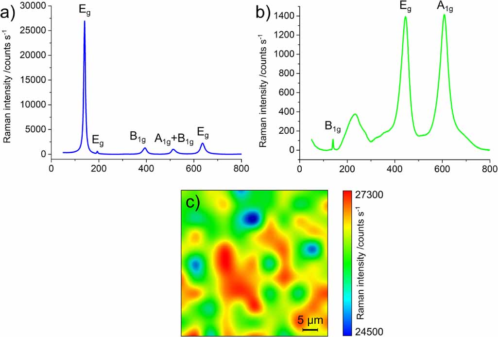
Anatase and rutile exhibit strong Raman scattering in the 100 cm−1 to 900 cm−1 spectral region [17–20]; in table 1, the major Raman bands in this region are reported. Figures 1(a) and (b) show Raman spectra of pure anatase and rutile, acquired on specimens employed in this study after sample preparation as illustrated in section 2.3, and in the experimental conditions described in sections 2.4–2.6. While the Raman spectra of these two TiO2 polymorphs are quite distinct from each other and easily identifiable in their pure forms, their spectral features overlap in mixtures: this is detrimental for their accurate relative quantification, especially when the amount of one of the two phases is small. Moreover, the intensities of the highest peaks in the same acquisition conditions differ significantly, impairing the sensitivity of the technique for rutile when mixed with anatase, and complicating the methodology of quantification.
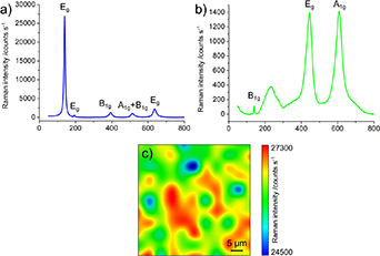
Figure 1. Raman spectra of anatase (a) and rutile (b) polymorphs, and Raman spatial map on an anatase flat film colored by the intensity of the 144 cm−1 peak (c) (11 × 11 pixels, 532 nm excitation wavelength, 4× microscope objective).
Download figure:
Standard image High-resolution imageTable 1. Vibrational frequency assignments (in relative wavenumbers, cm−1) of the bands in the spectral region employed in this study [17–20].
| Polymorph | Assignment | Raman shift/cm−1 |
|---|---|---|
| Anatase | Eg | 144 |
| Eg | 197 | |
| B1g | 400 | |
| A1g, B1g | 519 | |
| Eg | 640 | |
| Rutile | B1g | 143 |
| — | 235 | |
| — | 300–380 | |
| Eg | 447 | |
| A1g | 612 |
Another issue for reproducible optical spectroscopic quantification of powders is the variability of the Raman signal intensity, which can vary even for the same sample in the same experimental apparatus because of microscope focus, instrumental calibration and thermal fluctuations, spectral noise and background. As an example, figure 1(c) shows a 2D Raman spatial map on an anatase flat film, colored by the area of the most intense anatase Raman band (Eg at 144 cm−1). In spite of being a flatly-deposited film sample made from a well-pulverized single type of powder, there are noticeable fluctuations even in a single map of the most intense band.
An additional complication emerges from the nature of the sample: TiO2 powders vary greatly in powder compaction, particle size distribution, and granule arrangement, resulting in a heterogenous mixture with density and roughness that vary discontinuously within the sample. The issue is exacerbated in mixtures because of different mass densities for anatase and rutile (3.8 g cm−3 and 4.2 g cm−3 respectively) [6, 21], the preferential location of particles [22, 23], and the auto-agglomeration phenomena that arise among sub-micrometer particles in powders and suspension [24], which further limit the reproducibility of measurements of TiO2 powders, unless a definite protocol and standard procedures for sample preparation and testing is optimized to overcome local inhomogeneities.
For these reasons, traditional peak analysis on single spectra with a focus on one characteristic band for each polymorph can be misleading, and yields poor results in terms of accuracy, repeatability and reproducibility. Therefore, the interlaboratory comparison presented in this paper, which aimed at providing a standardized method designed to minimize sample and measurement variability, and assessing the reproducibility of the experiments with different Raman spectrometers and operators is urgently needed. The robustness and potential of this procedure was challenged further by using actual commercial powders with a broad particle size distribution as pure materials for the sample preparation.
In particular, to overcome these issues, the following steps were undertaken in producing and measuring the anatase–rutile binary mixtures:
- a sample deposition protocol based on suspension in acetone and sonication was adopted and optimized to homogenize the two phases and minimize the intra- and inter-variability in spatial distribution and composition of the specimens;
- Raman images over relatively large areas with respect to the dimensions of the investigated particles with low magnification and numerical apertures (NAs) objectives were acquired and averaged, instead of measuring single spectra;
- multivariate analysis on the spectral range of maximum Raman activity of the two polymorphs was employed, and the effect of data preprocessing on the final result was investigated.
With these conditions, the data provided by each participant in the ILC resulted in a root mean squared error lower than 5% in predicting the binary ratio of the two polymorphs in blind samples, i.e. with unknown composition.
2. Experimental
2.1. Experiment flow chart
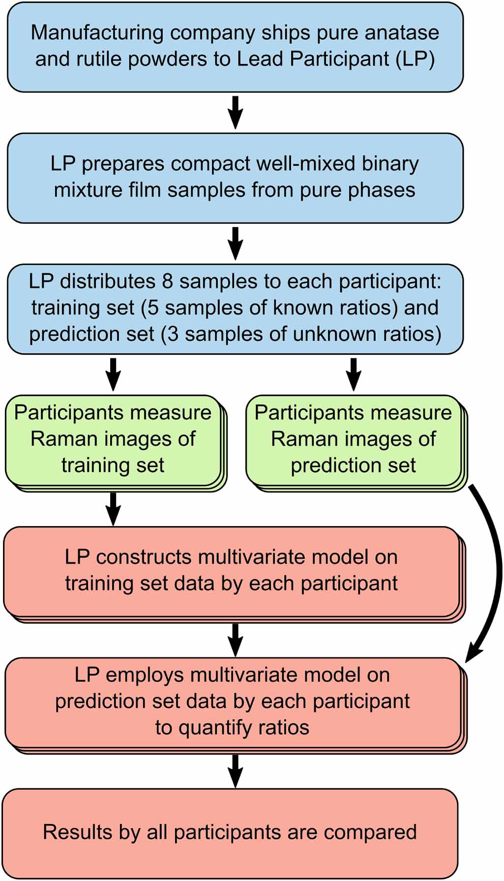
Figure 2 shows a flow chart of the steps for sample preparation, distribution, measurements and data analysis.
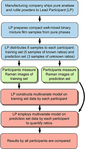
Figure 2. Flow chart representing the manufacturing and distribution of the samples (in blue), measurements of the data sets by each participant (in green) and data analysis (in red). Parallel processes on different data sets are represented by stacked boxes.
Download figure:
Standard image High-resolution imageCommercial powders were provided to the LP. The LP then prepared the samples and distributed them to all participants. The participants received eight samples divided into a training set (known concentration ratios) and a test set (unknown concentration ratios) and measured them according to the protocol (see supplementary information (SI)). The data were then sent to the LP for analysis: for each participant, the data were preprocessed; then the training set was employed for the construction of a multivariate model, which was used to quantify the unknown samples with the rest of the participant data. The results of all quantifications were then compared.
2.2. Materials
Anatase and rutile pure commercial powders were received from KRONOS Worldwide Inc. The specific commercial names of the materials were 'KRONOS 1171' (K1171, anatase) and 'KRONOS 2971' (K2971, rutile), both registered as E171 foodstuff colorants [21]. The powders were characterized as having a TiO2 content ⩾99% according to DIN EN ISO 591 [25]. The samples that were selected are not nanomaterials after the recommendation for classification of the European Union. The d50 (median value) of number-based primary particle size distribution measured by scanning electron microscopy (SEM) [26] lies above 100 nm for both pigments—although both pigments have a minority number of particles with diameters below 100 nm. Among the primary particles, pigments also contain lots of aggregates of primary particles. Both particle fractions in sum deliver a particle size distribution between 30 nm and 800 nm with a d50 of about 180 nm for K1171 and a d50 of about 210 nm for K2971 (see appendix B in the SI for SEM-based particle size distribution results).
2.3. Samples preparation and dissemination
Samples were prepared by the LP before dissemination. Pure powders and mixtures were prepared by gravimetric methods (using a Mettler Toledo Analytical Balance, model XS205DU, with 0.1 mg precision and repeatability of measurement in the relevant weight range between 0.020 mg and 0.025 mg). Approximately 10 g in total for each ratio was weighed with an analytical balance and deposited inside 50 ml falcon vials. The expanded uncertainty on the composition fractions was calculated to range from 0.01% to 0.001% depending on the proportions. The vials were then filled with acetone (spectroscopy grade, purity ⩾ 99.9%, by Carlo Erba) up to approximately 35 ml; each vial was then put in an ultrasonic bath (Qsonica Q700, frequency 20 kHz) for 10 min at 80 W. The suspensions were then left in a fume hood at ambient temperature for acetone to evaporate until approximately 10 ml of suspension remained; at this point, each vial was put again in the sonication bath (same settings as before) for 5 min. The resulting suspensions of dispersed, well-mixed particles were collected with a micropipette and deposited in acetone-resistant, multi-well sample holders (µ-Slide 8 well glass bottom sample holders, manufactured by ibidi), and left in the fume hood in order for the remaining acetone to completely evaporate. The resulting samples were macroscopically flat, compact, with visually uniform TiO2 films adhering at the bottom of the sample holder wells, which were then shipped to the participants. The films were not removed from the sample holder or manipulated in any way before or during measurements.
Each participant received five 'training set' samples of known anatase/rutile ratio, and three 'test set' samples on the ratios of which no information was attached. The training set was composed of the following binary mixtures: 100% anatase (named A100), 100% rutile (R100), 75% anatase + 25% rutile (AR7525), 25% anatase + 75% rutile (AR2575), and 50% anatase + 50% rutile (AR5050). The prediction set consisted in the following compositions: 45% anatase + 55% rutile (named X1), 80% anatase + 20% rutile (X2), and 5% anatase + 95% rutile (X3). Images of the sample holder containing the binary mixtures are shown in figure 1 of the measurement protocol, attached as appendix A in the SI.
2.4. Measurement setups and conditions
The participants were asked to perform Raman spectroscopic images in a backscattering configuration on the surfaces of the films with a 532 nm excitation laser wavelength; if this was not possible, the nearest excitation line was to be employed. The optimal spectral range of interest was [75 cm−1; 1000 cm−1] (Stokes scattering); the required average spectral resolution in that range was 5 cm−1 or less. The final spectral range employed in the multivariate analysis was [150 cm−1; 750 cm−1].
A low magnification, low NA microscope objective was optimal for the study: it was asked, if possible, to employ a 20× (or lower) magnification objective, with NA ⩽ 0.45; in confocal microscopes, a large confocal aperture was employed. In this way, a larger volume was investigated with each spectrum.
The participants were asked to perform spectral calibration on the Raman setups in the range of interest for the study. For wavelength calibration, the rare gas lamp method was chosen, in which a spectrum of the lamp is acquired with the Raman laser off, and the resulting emission peaks of the gas are then compared to tabulated data on the gas emission bands, as illustrated in ASTM E2529-06 ('Standard Guide for Testing the Resolution of a Raman Spectrometer') [27]. The pixel-to-wavelength relationship so established was used with the known laser wavelength to obtain the corresponding relative wavenumbers pertinent to the Raman spectra. Intensity calibration was carried out by the participants by their usual laboratory practices before each measurement session.
2.5. Measurement protocol
The complete measurement protocol is attached to the SI as appendix A.
Each single measurement was defined as the average of a Raman map; three measurements for each film were required, which were taken in different areas of the surfaces. Each image was required to have the same spatial parameters, to have dimensions of 20 µm × 20 µm or larger, with a step size of 2 µm or more, and comprised of at least 11 × 11 points (121 points in total). Measurements were performed in ambient conditions without further sample preparation.
The first part of the measurement protocol was the assessment of the optimal excitation power, which was then to be maintained constant throughout the measurements. The maximum admissible power at the sample was 1.0 mW. However, since the 144 cm−1 Eg anatase peak has a much higher intensity than the rest of the spectral features for both anatase and rutile, a single point Raman test was carried out by each participant focusing on the pure anatase sample surface, optimizing the excitation power and the acquisition time of the spectrum to avoid saturation of the spectrograph detector while achieving a good signal to noise ratio (S/N > 10) on the other Raman signals; in particular the 400 cm−1 B1g anatase spectral band was chosen as indicative of the rest of the major bands in the two polymorphs.
After the laser power and acquisition times were decided, the three subsequent image measurements were carried out on each sample. The raw spectra in the raster scans were averaged and then sent to the LP for data analysis.
2.6. Participating laboratories and setups
In table 2, the experimental setups and measurement parameters employed by the participants are reported.
Table 2. Experimental setups and parameters employed by the participants.
| Participant code | Raman spectrometer manufacturer and model | Excitation wavelength/nm | Objective magnification | Objective numerical aperture | Laser power/mW | Exposure time (number of exposures × single exposure time) | Sample identification number |
|---|---|---|---|---|---|---|---|
| A | WITec™ Alpha 300 S | 532 | 50× LWD | 0.55 | 0.8 | 1 × 1 s | 1 |
| B | Horiba LabRam HR Evolution | 532 | 10× | 0.25 | 0.44 | 1 × 0.5 s | 2 |
| C | Horiba LabRam HR Evolution | 532 | 10× | 0.25 | 0.6 | 1 × 3 s | 3 |
| D | WITec™ Alpha 300 A/R | 532 | 10× | 0.30 | 0.5 | 1 × 1 s | 4 |
| E | Thermo Scientific™ DXR™xi | 532 | 4× | 0.10 | 0.5 | 50 × 0.2 s | 5 |
| F | Horiba LabRam HR 800 | 457 | 10× | 0.25 | 0.13 | 25 × 0.2 s | 6 |
| G | WITec™ AR300 | 532 | 5× | 0.12 | 0.5 | 1 × 1 s | 7 |
| H | Renishaw inVia™ | 514.5 | 20× | 0.4 | 0.4 | 10 × 0.2 s | 8 |
| I | Renishaw inVia™ | 532 | 50× LWD | 0.5 | 0.5 | 1 × 0.5 s | 3 |
| J | BWTEK i-Raman | 532 | 20× | 0.4 | 0.3 | 2 × 1 s | 7 |
| K | Custom-made (Teledyne Princeton Instruments SP2500i spectrograph and Andor DU970N-BV CCD) | 532 | 20× | 0.25 | 1.0 | 1 × 12 s | 9 |
Nine sample sets were disseminated among 11 participants: most participants analyzed a unique sample, while sample 3 and 7 were employed for two datasets each due to logistic reasons. The excitation wavelength in most setups was 532 nm, while two of them used 514 nm and 457 nm. Most participants employed microscope objectives of magnifications equal to or lower than 20×, and NA ⩽ 0.4; two setups utilized 50× objectives with NAs of 0.5 and 0.55. Total exposure times for each Raman image ranged from 1 min to 25 min (average ≈ 7 min).
2.7. Multivariate analysis
PLS regression was employed in this work as the multivariate statistical model for the quantification of sample composition [10]. In PLS analysis, a linear regression model is calculated as an equation between the observed variables (predictors) and the predicted variable(s) after projection of the variables into new spaces. The parameters of this projection are calculated by maximizing the covariance among the input variables: the resulting variables are named latent variables (LVs), linear combinations of the original variables, whose weight (amount of influence) on each LV is represented by a vector called the loading vector. The higher the value of an original variable in the loading vector pertaining to an LV, the more its value for each data point influences that LV. Not all LVs are relevant for the model: therefore, as a dimensionality reduction procedure, only a handful of the LVs which explain the most variance are employed, and the others are discarded. Consequently, the original variables (spectral frequencies) with the highest (in absolute value) weight in loadings vectors for the employed LVs affect the final result the most and are therefore the most representative spectral regions.
In this work, the original input predictors were the Raman spectral intensities at each acquired wavenumber, and the predicted variable was the anatase component fraction in each sample. Therefore, the LVs were not actual spectra, but 'spectral-like' vectors evidencing the spectral features of most interest for the quantification of the two polymorphs. In the presented study, only the two to three LVs explaining the most variance were considered: this value was chosen for each dataset according to the results of cross-validation of the model in the training/optimization phase. The five calibration samples that constitute the training set were employed at this stage, with their actual anatase content as the predicted variable vector.
Before analyzing data, the input raw Raman spectra were preprocessed in order to improve their quality and allow better performance of the models. Firstly, the spectral ranges were cropped to an interval of [150 cm−1; 750 cm−1]. After this, mean centering was applied to data [28], i.e. for each dataset, the mean was calculated for each variable across all data, and this value was subtracted from the respective variable among every spectra. At this point, extended multiplicative scattering correction (EMSC) was eventually applied to four datasets to flatten the baseline in the samples and correct the random variations in light scattering—which arise because of uncontrollable fluctuations in the physical properties of the samples (e.g. particle size distribution) and experimental setup parameters leading to spectral variations not representative of actual changes and differences in the analytes—in order to improve the performance of these models [29]. Second order polynomial fitting was sufficient to obtain a straightforward scattering correction of the considered dataset and to obtain quantification accuracy and precision comparable with the other datasets, which do not need this specific preprocessing step.
After a PLS regression model was constructed from the preprocessed datasets of each participant (training phase, also known as model calibration phase), the models were applied for the quantification of the unknown samples (prediction phase). At this stage, no information on the actual amount of the two polymorphs in the prediction set samples was inserted into the models: this information was employed in the following phase of the ILC study, when the validity of the models from the measurements from each participant were assessed and compared with one another. Multivariate analysis was performed with PLS Toolbox from Eigenvector Research, Inc. (Manson, WA, USA) software for Matlab R2015a (MathWorks, Natick, USA).
2.8. Model performance metrics
Several parameters and figures of merit can be calculated and compared to validate a PLS regression model and evaluate its performance [30–32]. This can be carried out with or without a dataset left out of the model construction (holdout dataset) for verification; in this work, both strategies were employed, whereas, especially given that the number of variables was high, there was a tangible risk of overfitting. For each participant, in the model construction phase (in which only the training datasets were used), leave-one-group-out cross-validation was performed, where a group was defined as the set of three measurements on the same sample. After the parameters were chosen based on this method, a further verification on the prediction of the unknown ratios datasets was accomplished.
The following metrics were calculated for each model:
- RMSEC: root mean square of error in calibration (lower is better);
- RMSECV: root mean square of error in cross-validation (lower is better);
- RMSEP: root mean square of error in prediction (lower is better);
- R2: coefficient of determination (closer to 1 is better);
- Discrepancy: how close the measured/calculated data are to the true value of the measurand for the samples, calculated as
 (with the symbol c indicating the concentration fraction, meaning the average c, and the pedices measured and nominal referring to the output of the model and the concentration at which the sample was prepared respectively) for each test sample, and for the whole dataset as the average of the discrepancies for all test samples (lower is better)
11
;
(with the symbol c indicating the concentration fraction, meaning the average c, and the pedices measured and nominal referring to the output of the model and the concentration at which the sample was prepared respectively) for each test sample, and for the whole dataset as the average of the discrepancies for all test samples (lower is better)
11
; - Standard uncertainty: how much the prediction data are dispersed, calculated as the standard deviation of the three replicates of the prediction results for each test sample, and the overall reported value as the average of these (lower is better);
- LOD: limit of detection, calculated as (with indicating the average predicted result for 0% by the model, while is three times the standard deviation of the predicted results for 0% concentration, each for the specified TiO2 polymorph) (lower is better);
- LOQ: limit of quantification, calculated as (with indicating the average predicted result for 0% by the model, while is ten times the standard deviation of the predicted results for 0% concentration, each for the specified TiO2 polymorph) (lower is better).


In these metrics, 'errors' are intended as the residuals of the data points compared to the model prediction in the specified phase.
3. Results and discussion
3.1. Data preprocessing effects
The models were first constructed by employing the same preprocessing procedures for all participants data, and then for each dataset an optimal amount of LVs was selected on the bases of the minimization of RMSECV and cumulative explained variance (i.e. LVs explaining only fractions of percentage points of the total variance were not considered). In total ten datasets employed two LVs, since the addition of more LVs resulted in negligible improvements or even decline of RMSECVs, while one model received three LVs as input in order to achieve significantly better performance.
Analysis of data in a broader spectral range including the region around 144 cm−1 was initially carried out on several datasets. This resulted in noticeably worse RMSECVs with respect to the [150 cm−1; 750 cm−1] range eventually employed for the final study. Probable causes of this are the following. First of all, the much higher intensity of the 144 cm−1 Eg band of anatase can dominate the rest of the spectrum; here, input data were not scaled in order to bring each predictor to unit variance (i.e. standardization of data, or autoscale) in order to give more intense Raman signals higher impact in the model. The much larger intensity of this Raman peak hence weighted much more in the LVs calculation than any other signal. Furthermore, this discrepancy in intensity translates into a larger noise and variance in this region, which again was not scaled and could overshadow meaningful differences in other bands. Additionally, a possible issue could be the fact that both anatase and rutile Raman spectra feature a signal in this region, which could confuse the model. Consequently, the final data cropping excluded the 144 cm−1 region.
PLS models with preprocessing comprised solely of range cropping and mean centering before LVs construction and selection yielded good results (RMSEP < 5%) on most datasets. However, four datasets models (participant codes A, C, H, K) resulted in 5% < RMSEP < 10%, which was deemed not acceptable; these data visibly presented some systematic baseline differences for the various samples. Therefore, EMSC was applied to them after mean centering and before LVs construction. This method resulted in PLS models for these datasets with RMSEP < 5%. Other preprocessing methods were attempted for this purpose (such as first derivatives of the samples, applying Savitzky–Golay filters of first or second order, and subtracting baselines constructed from set anchor points), but this did not produce substantially better results with respect to EMSC, which has the advantage of being an algorithmic procedure with fewer free parameters—an important characteristic in order to use it for comparisons and standardization applications. It was found that applying EMSC to all datasets did not worsen the final results. Therefore, in the usage of Raman–PLS for this application, it is suggested to employ this method if the RMSEP were unsatisfactory, but also if the convenience of avoiding the preprocessing optimization step is sought, or if the user is not familiar with multivariate datasets preprocessing.
In section S2 of the SI, raw data and preprocessed data for each participant are shown.
3.2. Multivariate models training
Predictably, the loading vectors corresponding to the first LV of each model were, in absolute value, most intense in the Raman shift regions of the characteristic Raman bands of anatase and rutile; the loadings were of opposite signs for anatase and rutile active spectral regions, meaning that the final scores were most affected by these and shifted toward higher or lower quantities based on these in a way consistent with conventional Raman band analysis.
No evidence of particular similarities due to the utilization of the same sample in different setups, nor systematic differences between setups depending on excitation wavelengths, microscope objective magnifications, NAs, laser powers or exposure times were found.
Leave-one-concentration-out cross validation was performed after model construction. In table S2 in the SI, figures of merit (RMSEC, RMSECV and R2) regarding model calibration and cross validation are reported. In the figures in section S2 of the SI graphs representing loadings, PLS regressions, training and prediction datasets are reported for each model.
It is worth noting that, while in this study the quantification of unknown samples by the trained models was used as a measure of validity of the proposed Raman–PLS approach with the sample preparation and preprocessing illustrated here, the practice of measuring a separate dataset and using it in a prediction phase successive to cross validation (which is generally employed for model optimization) is always recommended before actual in-field application: this is a common practice in chemometrics and it is considered very important to avoid unexpected biases and overfitting, and to confirm robustness of the method in quantifying new samples.
3.3. Quantification of unknown samples: results comparison and Raman–PLS method performance
RMSEP and R2 for the prediction phase of the study are reported in table S2 in the SI. No participant stood out in terms of these parameters, after EMSC was applied. R2 values in prediction were all higher than 0.980; all RMSEPs were under 4.5%, and the vast majority were under 3%.
In table 3, the prediction results of the models on the test datasets are reported for each of the three unknown samples as the average of the three replicates and the corresponding standard deviation; the disparity between the predicted (average) value and the true (as prepared by gravimetry) anatase content is also shown as the prediction error. Figure 3 shows the plotted results of the ILC as deviations from the true value (prepared samples compositions, gravimetrically measured) of relative anatase content percentage in the samples 12 .

Figure 3. Comparison of the prediction results from the PLS models constructed from the datasets of the various participants, on the three unknown samples. (a): anatase content 5%; (b): anatase content 45%; (c): anatase content 80%. Error bars represent the expanded uncertainties from the three repeated measurements on each sample12; the red dashed lines indicate the anatase percentage fraction in each specimen.
Download figure:
Standard image High-resolution image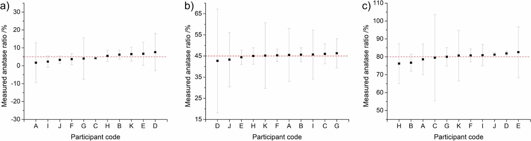
Table 3. Results of the quantification of the unknown samples (prediction phase) of the ILC. All values are expressed as percentages of anatase fraction in the samples. Prediction error is calculated as the difference between the average predicted values and the actual sample concentration.
| Anatase fraction/% in mass | Participant code | Prediction average/% in mass | Prediction standard deviation/% in mass | Prediction error/% in mass |
|---|---|---|---|---|
| 5 | A | 1.7 | 2.6 | −3.3 |
| B | 6.16 | 0.60 | +1.16 | |
| C | 4.242 | 0.052 | −0.758 | |
| D | 7.6 | 2.4 | +2.6 | |
| E | 6.7 | 1.5 | +1.7 | |
| F | 3.66 | 0.73 | −1.34 | |
| G | 4.0 | 2.7 | −1.0 | |
| H | 5.49 | 0.72 | +0.49 | |
| I | 2.31 | 0.74 | −2.69 | |
| J | 3.32 | 0.47 | −1.68 | |
| K | 6.47 | 0.89 | +1.47 | |
| 45 | A | 45.5 | 2.9 | +0.5 |
| B | 45.64 | 0.78 | +0.64 | |
| C | 46.0 | 1.1 | +1.0 | |
| D | 42.7 | 5.7 | −2.3 | |
| E | 44.45 | 0.80 | −0.55 | |
| F | 45.30 | 0.69 | +0.30 | |
| G | 46.3 | 1.6 | +1.3 | |
| H | 45.02 | 0.91 | +0.02 | |
| I | 45.7 | 2.7 | +0.7 | |
| J | 43.3 | 3.0 | −1.7 | |
| K | 45.2 | 3.6 | +0.2 | |
| 80 | A | 78.6 | 2.0 | −1.4 |
| B | 76.7 | 1.1 | −3.3 | |
| C | 79.5 | 5.6 | −0.5 | |
| D | 81.91 | 0.17 | +1.91 | |
| E | 82.6 | 3.3 | +2.6 | |
| F | 80.76 | 0.84 | +0.76 | |
| G | 80.0 | 1.2 | 0.0 | |
| H | 76.2 | 2.6 | −3.8 | |
| I | 80.9 | 1.4 | +0.9 | |
| J | 81.17 | 0.27 | +1.68 | |
| K | 80.7 | 3.6 | +0.7 |
It can be observed that the average predicted value distributions are not skewed in any direction for all samples, indicating that was no evidence of systematic overestimation or underestimation biases of the method. Indeed, the average of these values were 4.7%, 45.0%, and 79.9%, very close to the respective reference values of 5.0%, 45.0% and 80.0%. The standard deviations of the estimations by the participants were varied and random, and they did not appear to follow particular trends with respect to specific participants, experimental setups characteristics, or sample compositions.
The effectiveness of the models and their generalized capabilities can be summarized by a number of calculated parameters. In table S3 in the SI, for each model, values of discrepancy, standard uncertainty, LOD and LOQ are reported. Discrepancy values were found to be all below 2.0%, and standard uncertainty values below 3.0%. LODs for anatase resulted to be under 5.5% for all regressions, with most models achieving LOD ⩽ 2.0%. For rutile, the values were significantly higher, with six participants achieving LOD < 5.0%, but five of them attaining 5.0% < LOD < 10.0%. Indeed, LODs and LOQs of 9 out of 11 models were higher for rutile than anatase: since these figures of merit were determined by the performance of the regression applied in the respective regions of low amounts, it follows that these findings imply that the method likely operates better at low anatase concentrations than at low rutile fractions. In table 4, overall discrepancies and standard uncertainties of the models for all participants are reported, calculated as described in section 2.8.
Table 4. Overall discrepancies and standard uncertainties of the computed models on every dataset.
| Participant code | Discrepancy/% | Standard uncertainty/% |
|---|---|---|
| A | 1.7 | 2.5 |
| B | 1.7 | 0.8 |
| C | 0.8 | 2.2 |
| D | 0.7 | 2.8 |
| E | 1.6 | 1.9 |
| F | 0.8 | 0.8 |
| G | 0.8 | 1.8 |
| H | 1.4 | 1.4 |
| I | 1.4 | 1.6 |
| J | 1.5 | 1.2 |
| K | 0.8 | 2.6 |
With the experimental setups and measurement conditions reported in table 2, the S/N were high enough not to affect the final quantification results, and no correlations were found between S/N values and quality figures of the PLS regressions and quantifications. Therefore, it can be assumed that the Raman spectroscopy exposure times for each spectrum could be reduced without significantly impacting the performance of the techniques presented here, decreasing the total time of analysis. Moreover, this could allow the number of points and physical surface on each Raman map to increase, and/or increase the number of maps while maintaining similar times of analysis. This would further reduce data dispersion, which during prediction affects the calculation of standard uncertainty, LOD and LOQ, while also expanding the dataset to better estimate data uncertainty.
4. Summary and conclusions
This article presented the ILC conducted under the framework of VAMAS TWA 42 Project 2 [14]. This work involved 11 laboratories worldwide, operating diverse Raman micro-spectroscopy setups to verify the feasibility of Raman spectroscopy and multivariate modeling techniques for accurate quantification of industrially pure TiO2 anatase and rutile pigments in binary mixtures. This procedure supports with good efficacy some industrial and academic needs that, as of today, are covered normatively by measurement techniques requiring lengthy procedures whose performance decreases in ranges that are not close to purity of one of the two phases.
A careful preparation protocol for TiO2 powders was optimized and presented for the production of titania films of adequate homogeneous density which were found to be stable and apt for international transportation. A measurement procedure was also developed and introduced, involving Raman imaging to overcome local inhomogeneity and granularity of the TiO2 particles, by which a dataset suitable for model training and usage can be obtained in a short amount of time, and could potentially be further reduced if necessary. The effect of preprocessing on the final result of the multivariate analysis was explored with widespread model metrics, as was the effect of hyperparameters selection.
In conclusion, the ILC results presented in this paper demonstrate that the Raman–PLS approach can be successfully employed for the quantification of TiO2 polymorph content ratio in anatase–rutile binary mixtures with discrepancies with respect to the nominal values of less than 2% in the 5%–95% ratios range. Furthermore, the performance metrics of the PLS models constructed from most of the datasets suggest that further improvement over these figures is possible.
Acknowledgments
The authors would like to thank KRONOS Worldwide, Inc. [21] for supplying the titanium dioxide powders employed in sample preparation for this work. This work was conducted in the framework of VAMAS, as TWA 42 Project 2. This work was supported by the UK Government's Department for Business, Energy and Industrial Strategy through the National Measurement System. Commercial equipment, instruments, and materials are identified in this paper in order to specify the experimental procedure adequately. Such identification is not intended to imply recommendation or endorsement by the National Institute of Standards and Technology or the United States Government, nor is it intended to imply that the materials or equipment identified are necessarily the best available for the purpose.
Footnotes
- 11
Note that this is often named 'accuracy' in machine learning and other fields; however, this does not coincide with the metrological definition of accuracy as per its definition in the International Vocabulary of Metrology and its notes [30], nor exactly with its definition in DIN ISO 5725-1 [32], section 3.6; therefore, the term 'discrepancy' was chosen for the name of this quantity.
- 12
Expanded type A uncertainties uc(y), intervals encompassing 95% of the respective distributions, estimated from the standard deviations u(y) of the data multiplied by the coverage factor of the Student's t-distribution with 2 degrees of freedom at the indicated confidence level: uc(y) = u(y) × 4.30, as by annex G of the Guide for the Expression of Uncertainty in Measurement (JCGM 100:2008) [33].
Appendix_B_EM_images.pdf (0.4 MB PDF)
Appendix_B_Anatase_size_1.pdf (0.5 MB PDF)
Appendix_B_Anatase_size_2.pdf (0.5 MB PDF)
Appendix_B_Rutile_size_1.pdf (0.5 MB PDF)
Appendix_B_Rutile_size_2.pdf (0.4 MB PDF)
Appendix_A_Protocol.pdf (1.6 MB PDF)
Supplementary_information.pdf (3.1 MB DOCX)