Abstract
We investigate the population and several properties of radio pulsars whose emission does not null (non-nulling) through simulation of a large pulsar sample. Emission from a pulsar is identified as non-nulling if (i) the emission does not cease across the whole pulse profile, and (ii) the emission is detectable. For (i), we adopt a model for switching in the plasma charge density, and emission persists if the charge density is non-zero. For (ii), we assume that detectable emission originates from source points where it is emitted tangentially to the magnetic field-line and parallel to the line-of-sight. We find that pulsars exhibiting non-nulling emission possess obliquity angles with an average of 42 5, and almost half the samples maintain a duty cycle between 0.05 and 0.2. Furthermore, the pulsar population is not fixed but dependent on the obliquity angle, with the population peaking at 20°. In addition, three evolutionary phases are identified in the pulsar population as the obliquity angle evolves, with the majority of samples having an obliquity angle between 20° and 65°. Our results also suggest that emission from a pulsar may evolve between nulling and non-nulling during its lifetime.
Export citation and abstract BibTeX RIS
1. Introduction
The population and properties specific to radio pulsars that exhibit only non-nulling emission are unclear. Yet, pulsars with nulling behavior are well distinguished as a distinct type of pulsar (Wang et al. 2007; Konar & Deka 2019; Sheikh & MacDonald 2021). Identified shortly after the first pulsar was discovered (Backer 1970), nulling is a relatively common phenomenon that manifests as cessation in the whole pulse emission over a time that lasts from several rotation periods to minutes (Backer 1970; Rankin 1986; Wang et al. 2007; Young et al. 2015). So far, more than 200 pulsars have been reported with such behavior (Sheikh & MacDonald 2021). It is relatively straightforward to show that a radio pulsar is a nulling pulsar. All that is required are clear detections of several instances when there is no detectable emission. On the contrary, it is difficult to show that a pulsar is not a nulling pulsar (Rankin 1986), referred to as an emission non-nulling pulsar in this paper (or simply a non-nulling pulsar where there is no confusion). Observationally, there is no telling whether or not the thus-far continuous emission from a pulsar would be interrupted in subsequent pulses. One difficulty lies with the similarities in the emission properties (when not nulling) and the rotation characteristics between the two types of pulsars. Therefore, it is challenging to predict whether a pulsar will exhibit non-nulling emission based only on its rotation or emission characteristics. Nevertheless, there were many investigations into the properties of nulling, which also offered hints on certain properties for pulsars that should not exhibit nulling. For example, the suggestion that null pulses appear to increase with the pulsar's age also implies that pulsars with large age are less likely to exhibit non-nulling. Ritchings (1976) concluded that nulling is related to the rotation period of a pulsar, such that pulsars with longer periods should null more often (Biggs 1992; Wang et al. 2007). There were also studies suggesting that half of the known pulsars should demonstrate nulling, which also imply that half of the known pulsars may be non-nulling. There were predictions that the frequency of null is related to the morphology of the integrated profiles (Biggs 1992). By separating profiles into different classes, Rankin (1986) showed that pulsars with pulse profiles having a single component should null less frequently (Weisberg et al. 1986) than pulsars possessing profiles with multiple components. Biggs (1992) further suggested that a pulsar would null more when its obliquity angle, α, evaluated between the rotation and magnetic axes, is small. However, a statistical study of nulling pulsars concluded that nulling shows less correlation with the obliquity angle or the rotation period but more with the profile width (Li & Wang 1995). This indicates that nulling, and non-nulling, may also be related to the emission geometry.
The purpose of this paper is to investigate several characteristics of emission non-nulling pulsars through studies of the distribution of α, β and different profile widths, or duty cycles, δ, from simulation of a large pulsar sample. Here, β = ζ − α is the impact parameter, and ζ is the viewing angle between the rotation axis and the line of sight (Radhakrishnan & Cooke 1969). There are two criteria for confirming a radio pulsar as an emission non-nulling pulsar, namely (i) its emission does not cease or cessation does not occur across the whole pulse profile, and (ii) its emission must be detectable. Point (i) involves the knowledge for changes in the pulsar radio pulses between emission (non-nulling) and nulling. An important source of such information comes from the consideration of the quasi-periodic emission switching in intermittent pulsars between pulse "on," when emission is detectable, and "off," in which the emission ceases (Kramer et al. 2006; Camilo et al. 2012; Lorimer et al. 2012; Lyne et al. 2017). The mechanism of the phenomenon can be interpreted as changes in the emitting plasma density between two states of ample and vacuum (Kramer et al. 2006). This implies correlation between radio emission and the plasma density, and pulse cessation arises when the plasma density is zero. The correlation is consistent with the common view that pulsar radio emission is produced from ultra-relativistic plasma out-streaming along the open field-lines in two-stream instability, which leads to the prediction that the pulse intensity is proportional to the plasma density (Manchester & Taylor 1977; Cordes 1979; Lyubarskii 1996). Although there is still no commonly accepted model for changes in the plasma density, a model for multiple quasi-stable emission states, each with different plasma charge densities, has recently been proposed for obliquely rotating pulsar magnetospheres (Melrose & Yuen 2014). The model is based on synthesis of two limiting conditions for plasma charge density. One limit corresponds to a corotating magnetosphere, in which the plasma charge density maintains the Goldreich & Julian (1969) value, ρGJ. Another limit refers to the vacuum-dipole model, in which the origin of the inductive electric field,
E
ind, is attributed to a rotating magnetic dipole. The need to screen the parallel component of
E
ind requires the presence of a charge density, denoted by  , that is arbitrarily small and insufficient to generate the potential field required by corotation. A class of synthesized models for emission states characterized by the parameter y is then constructed through consideration of the plasma charge density in each emission state as a combination of y and (1 − y) fractions of
  and ρGJ, respectively. Consequently, a change in the value of y would result in a change of the plasma charge density, which corresponds to a change in the emission state. It follows that the emission will persist in any emission states in which the plasma charge density is non-zero. In order for the changes in pulse emission to be detectable, the switching in the emission state must occur at the locations that are visible to an observer. Here, we adopt an emission geometry in which radiation is emitted from source points on the field-lines whose footpoints are located in the open-field region. Visible emission comes only from the source points (visible points) where the emission is directed tangentially to the dipolar magnetic field-lines (Cordes 1978; Hibschman & Arons 2001; Kijak & Gil 2003) and parallel to the line-of-sight direction. The location of a visible point in the magnetosphere for a pulsar phase, ψ, can be determined uniquely given ζ and α. As the pulsar rotates, the visible point moves tracing a closed path for every pulsar rotation, referred to here as the trajectory of the visible point. Changes in the pulse emission can be detected by an observer provided that the changes take place at the locations defined by the trajectory of the visible point.
The observations of more and more pulsars with detectable switching in the emission properties (Smits et al. 2005; Kramer et al. 2006; Rankin et al. 2006; Lyne et al. 2010, 2017; Camilo et al. 2012; Lorimer et al. 2012; Keith et al. 2013; Marshall et al. 2015; McSweeney et al. 2017) demonstrate that it is common for pulsar magnetospheres to undergo sudden changes of some sort. An essential piece of information from these observations is that the timescale for emission switching in different pulsars is different. It follows that the switching timescale in some pulsars may be too long to be captured in regular observing sessions. For our investigation, we assume that emission switching occurs in all our samples. From study of the polarization position angles based on a large sample of pulsars (Rankin 1993a; Tauris & Manchester 1998), the distribution of α was demonstrated to be situated within the range of α ≲ 90°, with the distribution occupying mostly small values (Rankin 1990). The result was reinforced by different simulations (Zhang et al. 2003; Kolonko et al. 2004). Hence for our samples in this paper, we select α values from the range between 1° and 90°. In addition, the width of the profile must be known to determine the emission across the profile. We consider duty cycles from 0.05 to 1 obtained from different pairs of ζ and α under an assumed maximum emission height. As for the last case, pulsar radio emission was shown to originate from a height at about 0.1rL (Johnston & Weisberg 2006), with rL = c/ω⋆ being the light-cylinder radius and ω⋆ the spin frequency of the star. In our simulation, a maximum height of 0.2rL is assumed. We also focus on emission from the main pulse without referring to the interpulse. Some pulsars were observed to demonstrate correlated changes between different emission features, such as subpulse drifting, nulling, quasi-periodic modulation, micro-structure and polarization properties (Taylor et al. 1975; Bartel et al. 1982; Rankin 1986; van Leeuwen et al. 2002; Janssen & van Leeuwen 2004; Redman et al. 2005), suggesting that variations in the radio emission may involve a more complex change in the emission process. Despite many investigations, such correlation between different emission phenomena is still largely uncertain and its relationship to the pulsar radio generation process remains unclear. There are also unconventional models for the pulsar emission process which involve unusual magnetic field structures (Gao et al. 2016, 2017) and a pulsar model with strange quark matter (Xu et al. 1999, 2001). Before including such complicated cases, it is useful to explore the implications of the traditional definition in an idealized model.
We outline the model for non-nulling emission in Section 2. The simulation procedures and the results are presented in Section 3. The analysis for the correlations between emission non-nulling pulsars and the pulsar parameters is shown in Section 4, and we discuss and conclude the paper in Section 5. The electromagnetic fields, the emission geometry and the transformation matrices referred to in the paper are outlined in Appendices A–C, respectively.
2. Model for Non-nulling Emission
Verifying the emission of a pulsar as non-nulling involves ensuring that the visible emission does not cease across the whole pulse profile in every rotation. In this section, we summarize the model presented by Melrose & Yuen (2014) with an emphasis on changes in plasma density in relation to the condition for non-nulling emission.
2.1. Detectable Changes in the Plasma Density
The interpretation of emission changes in intermittent pulsars as due to changes between two states of plasma density (Kramer et al. 2006) implies that different emission states, each with unique plasma density, are allowed in a pulsar magnetosphere. In the model for pulsar magnetospheres with multiple emission states (Melrose & Yuen 2014), the different emission states can each be identified by a particular value in the parameter y between two limiting conditions, designated by 0 and 1, respectively. The two conditions can be defined through the electric field in an obliquely rotating pulsar magnetosphere, which takes the form

where b is the unit vector along the dipolar field-lines. In Equation (1), E ind signifies the electric field induced by an obliquely rotating magnetic dipole, with the form given by Equation (A2), and the electric field associated with the corotation charge density is given by E pot = −∇Φcor. The limiting condition for y = 0 then corresponds to the corotation electric field, E = E cor, given by Equation (A5) as specified in the corotation model (Goldreich & Julian 1969), and the associated corotation charge density is signified by

The other limit, represented by y = 1, is associated with the "minimal" model, which is signified by the screening of the parallel component of the inductive electric field,
E
ind∥, while the perpendicular component,
E
ind⊥, has the same value as in the vacuum-dipole model. The screening requires a charge density,  , to generate an electric field such that
  . The
. The  takes the form given by

The necessity to screen the electric field parallel to the magnetic field-lines in every emission state for an oblique rotator demands a charge density, which has the form given by Melrose & Yuen (2014)

The screening is effective if the condition is met for the creation of the secondary particle pairs that result in a multiplicity, λ, larger than unity (Beskin et al. 1993; Melrose & Yuen 2012). The last case can be written as λ = e(n+ + n−)/ρGJ ≫ 1 (Gurevich & Istomin 2007), with ρGJ = e(n+ − n−) and n± being the number density of positrons and electrons. In our model, the plasma density is signified by  . The correlation between the pulse intensity and the plasma density (Manchester & Taylor 1977; Cordes 1979; Lyubarskii 1996) implies that the former is proportional to
  . Assuming the same λ across different emission states would mean that the pulse intensity is proportional to
  . It follows that a variation in the value of y corresponds to a change in
  , which results in a change of the pulse intensity.
The value of y, and the associated value of  , at given coordinates in a magnetosphere can be determined uniquely in an emission geometry defined by a pair of ζ and α. We adopt an emission geometry (see Appendix B) in which the magnetic field-lines are of a dipolar structure, and emission arises from source points on the field-lines whose footpoints are located within the open-field region (Cordes 1978; Kijak & Gil 2003). The condition for visible emission then requires that the emission be emitted tangentially to the local field-lines (J. A. Hibschman & J. Arons 2001) and in parallel to the line-of-sight. From such geometry, an explicit solution can be obtained for the source point of visible emission in terms of the polar and azimuthal angles as a function of ψ. In the magnetic frame, the angles are represented by θbV and ϕbV and their expressions are given by Equation (B1). Transforming to the observer's frame using Equation (C5), the visible point can be expressed in terms of the angles θV and ϕV relative to the rotation axis. For an oblique rotator, the visible point moves forming a closed path after one pulsar rotation, which is called the trajectory of the visible point. Figure 1 shows three examples for the trajectory of the visible point in the magnetic frame. Note that the size and shape of a trajectory vary depending on the values of ζ and α, and they are generally not circular and may or may not include the magnetic pole.

Figure 1. Plot illustrating three trajectories of the visible point using α = 25° and ζ = 10° (green), 30° (brown) and 60° (blue). The plot is constructed in the magnetic frame such that the magnetic pole is located at the origin. Both blue and brown trajectories enclose the magnetic pole. The boundary of an open-field region at 0.2rL is drawn in black dotted curve with its center located at the origin. Also shown is the non-nulling (gray) region for the same α. While all the trajectories cut the open-field region differently, only the brown and green trajectories traverse the non-nulling region, with the latter trajectory lying entirely inside both the open-field and non-nulling regions.
Download figure:
Standard image High-resolution imageThe assumption that emission originates from the open-field region implies the dependence of the visible point on height. Given a pair of ζ and α, there exists a minimum height, rV, at which the trajectory of the visible point is tangent to the locus of the last closed field-lines (see Appendix B). The height, rV, changes as a function of ψ as indicated by Equation (B2). To illustrate that, Figure 1 also shows an open-field region with a boundary (black dotted closed curve) at 0.2rL. All trajectories cut the open-field region but at different pulsar phases. For the blue trajectory, it enters the region at A, corresponding to ψ1 = −30°, and exits it at B, where ψ2 = 30°. The rest of the trajectory is located at heights that are above 0.2rL. Similarly, only the part of the brown trajectory between C and F lies inside the open-field region, with ψ1,2 = ∓94°, respectively, between which emission is visible. This is different for the trajectory in green, which lies entirely within the open-field region, meaning that the variation of height along the trajectory is always below 0.2rL and emission is potentially visible throughout the whole pulsar rotation. The range of pulsar phase for detectable emission is bounded by ψ1 and ψ2, and hence the profile width is given by Δψ = ψ2 − ψ1, or equivalently in duty cycle by δ = Δψ/2π. For the blue trajectory, Δψ = 60°, or δ ≈ 0.17, whereas it is Δψ = 188°, or δ ≈ 0.52, for the brown trajectory. The green trajectory, being completely enclosed in the open-field, has a Δψ = 360°, which gives δ = 1.
2.2. Geometry for Non-nulling Emission
We define non-nulling emission as visible emission that does not cease across the whole pulse profile in every pulsar rotation. For a pair of ζ and α, the angular locations of the visible point can be uniquely defined by the trajectory of the visible point. Then, Equation (4) is used to solve for the y value that satisfies  for each ψ = ψE between ψ1 and ψ2 that lies inside the open-field region. A pulsar sample is regarded as an emission non-nulling pulsar provided that no solution exists for
  with 0 ≤ y ≤ 1 at one or more ψE. This implies that the open-field region and the non-nulling region must contain overlaps and the overlapping regions must be cut by the trajectory of the visible point. Such relationship between the emission geometry and non-nulling emission is illustrated in Figure 1. The figure demonstrates a region (in gray) in which
  for 0 ≤ y ≤ 1. It is clear from the figure that the location for the non-nulling region is different from that for the open-field region. This implies that a trajectory that cuts the latter does not necessarily also cut the former. An example is the blue trajectory, with which it does not cut any part of the non-nulling region even though it lies partially in the open-field region. It follows that the emission along the blue trajectory does not satisfy our definition for non-nulling emission because it lies entirely in the region where
  exists for 0 ≤ y ≤ 1 (cessation across the whole profile). The brown trajectory traverses the open-field region from C to F, and cuts the nulling region only from D to E at ψ1,2 = ∓ 655. This means that the parts of the trajectory through CD and EF will always be emitting (cessation not occurring across the whole profile), and hence the pulsar would be regarded as an emission non-nulling pulsar. With δ = 1, the green trajectory is immersed completely in the open-field region, and visible emission occurs along the entire trajectory which also lies within the non-nulling region giving non-nulling emission detectable across the whole profile.
3. Simulation Procedures and Results
Our investigation of emission non-nulling pulsars and their correlations with the duty cycle (δ), the impact parameter (β) and the obliquity angle (α) is based on simulation of a large sample of pulsars. Below, we summarize the simulation procedures in relation to the criteria for identifying non-nulling emission.
In three-dimensional coordinates, the rotation axis of a pulsar and the line of sight of an observer are both random and uniform resulting in an isotropic distribution. We adopt a random distribution of the obliquity angle described by a cosine function (Smits et al. 2009). Furthermore, an emission from a pulsar is assumed to be beamed toward an observer, meaning that the values of β are dependent on the distribution of α. We assume the likelihood of the magnetic axis occurring in the direction of the line of sight being proportional to 1/4π. For our simulation, we consider the ranges of 1° ≤ α ≤ 90° and 0° ≤ ζ ≤ 90°. We also restrict β to within the value of ∣β∣ ≤ 15° for consistency with observations (Lyne & Manchester 1988), and apply an upper limit of r ≤ 0.2 rL for the emission height to all the samples (Johnston & Weisberg 2006). We assume that all the sample pulsars are emitting in an emission state with 0 ≤ y ≤ 1, and each is capable of emission state switching in association with changes in  . With these parameters defined, the non-nulling emission of a sample with a pair of ζ and α is determined at {θV, ϕV} for each ψ from −180° to 180°, in steps of 01, along the trajectory of the visible point using Equations (B1) and (C5). The values of ψ1 and ψ2 are determined, making sure that the heights are below 0.2rL, with the fiducial plane assumed to be at ψ = 0°. After that, violation of the condition for
  with 0 ≤ y ≤ 1 is checked for each ψE, between ψ1 and ψ2, using Equation (4). The pair ζ and α is labeled as non-nulling only if such violation is identified. We obtain a total of 357,395 samples for non-nulling and nulling pulsars.
Figure 2 shows the results of the distribution for the emission non-nulling pulsars for different δ, in steps of 0.05, from the simulation. For comparison, the corresponding distribution for nulling pulsars is also shown. We find that emission non-nulling pulsars exist for all δ from 0 to 1. Specifically, the proportion of non-nulling pulsars increases relative to that of the nulling pulsars as δ increases. The former dominates from δ ≳ 0.2, and it reaches 100% from δ = 0.4. We obtain 289,441 detectable samples, giving 81.0% of non-nulling pulsars. Overall, about 53% of the non-nulling pulsars have δ ≤ 0.2, and around 80% possess a duty cycle of ≤0.45. Comparing with the estimated δ ∼ 0.1 for ordinary pulsars (Kolonko et al. 2004; Maciesiak et al. 2011), our result indicates that the distribution of emission non-nulling pulsars contains relatively large duty cycles.
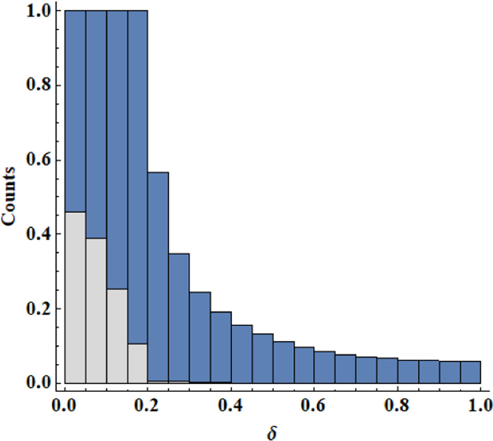
Figure 2. Histogram showing the normalized distributions of emission non-nulling (blue) relative to nulling (gray) pulsars for the 20 values of δ between 0.05 and 1.0.
Download figure:
Standard image High-resolution image4. Properties of Non-nulling Pulsars
In this section, we examine the relationships between non-nulling emission and each of β, α and δ, and the implications of the correlations.
4.1. Relations to the Emission Geometry
The variation in the distribution of α for emission non-nulling pulsars for ten different δ values is shown in Figure 3. As δ increases, the total number of non-nulling pulsars changes in such a way that it rises and reaches a maximum at δ ∼ 0.2, followed by a decrease and arriving at the minimum at δ = 1.0. At small δ, the distribution covers all the α values in our simulation. Beyond that, the number drops and reaches zero at α = 90°. As δ increases, the distribution undergoes significant changes from spreading over all the α values to increasingly shrinking to cover only a smaller range of α up to ∼25° at δ = 1.0. Furthermore, non-nulling pulsars are not found for α ≳ 30° from δ ≳ 0.4, whereas they always exist at α ≲ 30° for all δ. In addition, the total number under the distribution decreases considerably. A peak showing the most common α value is also clearly seen in each distribution, which shifts toward smaller α as δ increases. The last is consistent with the mean value of α that reduces as δ increases. For δ ≥ 0.5, the changes are mostly seen as a decrease in the total pulsar number and shrinking of the distribution, but the general shape of the distribution remains. This suggests a weaker dependence of the distribution on large δ.

Figure 3. Histogram showing the normalized distribution of α for ten different δ. The δ value increases from left to right and from top to bottom. The range of α under the distribution reduces as δ increases. The mean value of α for each distribution,  , is given for each δ.
Download figure:
Standard image High-resolution imageAn alternative presentation for the variation in the number of non-nulling pulsars as a function of δ for different α values is given in Figure 4. The α values are divided into nine consecutive intervals. For α between [0, 10)°, the pulsar number increases as δ increases from 0.05 to about 0.4, beyond which the number is almost constant. For α values up to about 20°, the number of non-nulling pulsars at large δ (>0.4) is more than that at small δ. This reverses as the values in an α interval increase, and the curves display a clear maximum that shifts increasingly toward smaller δ. Beyond the maximum, the pulsar number drops, but at a rate that is unique for different α intervals. The δ range under a curve reduces gradually as the values in an α interval increase. It begins with a non-zero pulsar number over all δ values (brown, blue and gray) to reach zero at a δ value that decreases as α increases. Note that almost similar changes occur for the two α intervals from 70° to 90°. It is apparent from Figures 3 and 4 that the number of emission non-nulling pulsars is dependent on both δ and α.

Figure 4. Plot showing variation of the normalized pulsar number counts for different intervals of α as a function of δ. The legend on the right indicates the nine intervals of α with a square bracket, and a parenthesis signifies the corresponding boundary value being included or excluded, respectively. Note that the curves for the two largest intervals are overlapped for δ ≳ 0.2.
Download figure:
Standard image High-resolution imageThe variation in the distribution of β is shown in Figure 5 for the same values of δ as in Figure 3. For all δ in our simulation, we find that there are always non-nulling pulsars that possess β ≤ 0°, with the amount being dependent on δ. However, the number of non-nulling cases with positive β increases as δ increases, but both +β and −β are never distributed evenly regardless of δ. This can also be seen from the mean value of β that displays increasingly positive behavior as δ increases in general, but never equals zero. Furthermore, the total number of pulsars is largest for δ ∼ 0.2 and decreases as δ increases.
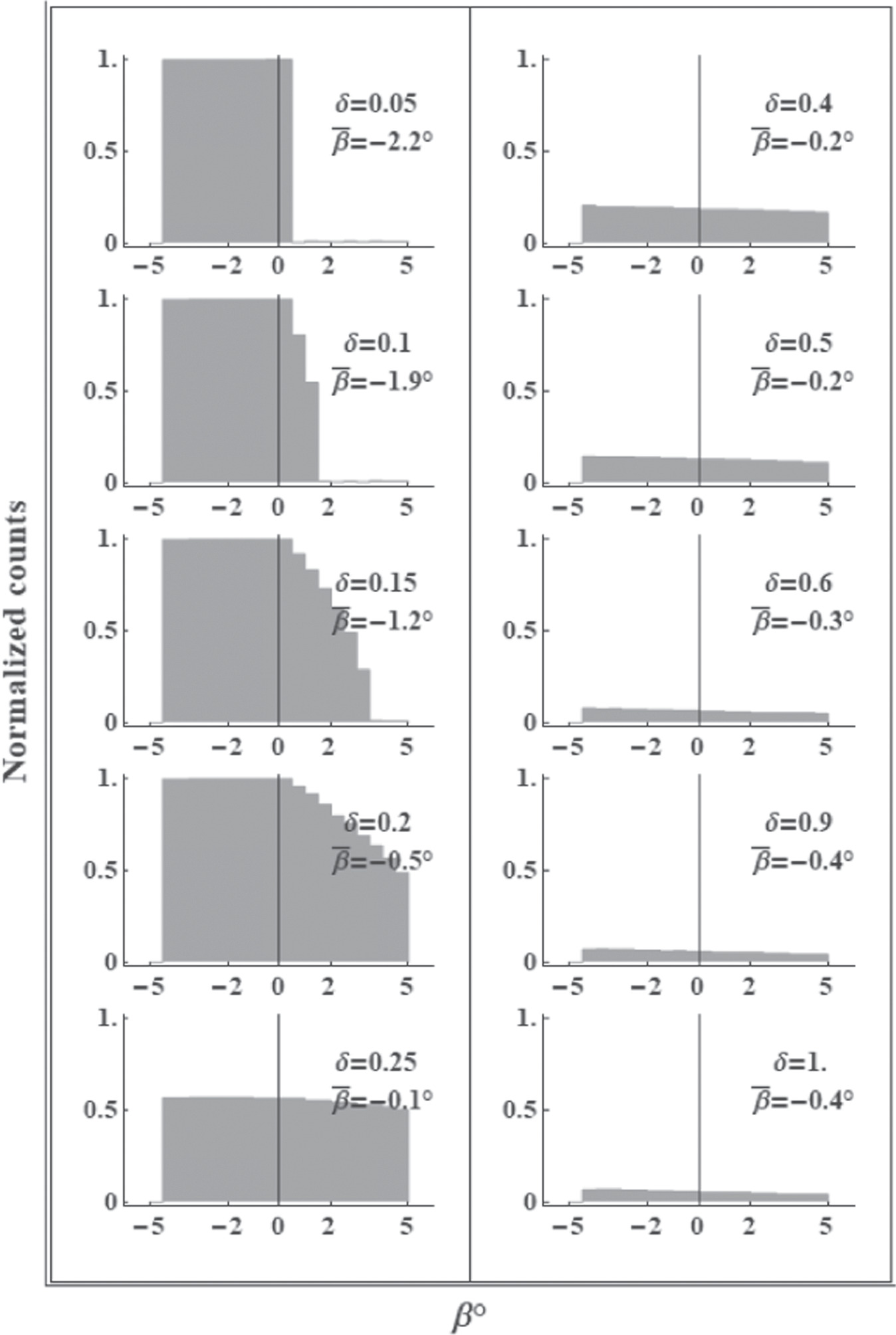
Figure 5. Similar to Figure 3 but for the normalized distribution of β showing their distributions that cover an increasingly broader range of β as δ increases. The mean value of β is given for each δ.
Download figure:
Standard image High-resolution image4.2. Evolution of the Correlation between Non-nulling and α
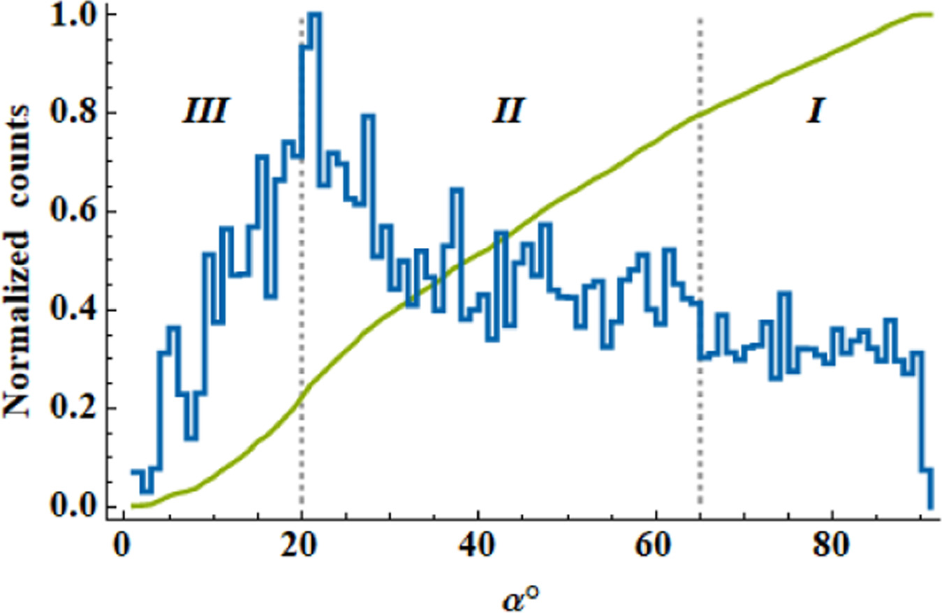
As displayed in Figure 3, the changes of covering all α at small δ to being increasingly concentrated around smaller α as δ increases imply that emission non-nulling pulsars with different δ show different preferences for α values. An alternative presentation is depicted in Figure 6, which shows a normalized distribution for the number of non-nulling pulsars as a function of α. Noticeable fluctuation is seen in the number of non-nulling pulsars across the α values, but an overall pattern can still be recognized. In general, emission non-nulling pulsars can be found for almost any α values in our simulation. However, the distribution varies in such a way that it possesses a certain number of non-nulling pulsars at α = 1°, which increases linearly as α increases and reaches a peak at α ∼ 20°. After that, the distribution decreases approximately exponentially as α increases up to about 65°, followed by a roughly constant distribution for the next 20°. It then drops again rapidly reaching zero at α = 90°. We find that 50% of the pulsars have α ≤ 395, and 80% possess α ≤ 66°, with the average for α being 425. This demonstrates that emission non-nulling pulsars tend to possess smaller α values, which is consistent with observations (Tauris & Manchester 1998). Also shown in Figure 6 is the normalized cumulative sum, as a green curve, representing a function of increasing α. In general, the slope of the curve is positive meaning that the cumulative count increases as α increases. However, the slope is not constant, and a rapid increase in number occurs at small α up to about 30°, followed by a slower increase as α increases further.
Figure 6. Plot showing variation in the normalized number of emission non-nulling pulsars as a function of α as a blue curve. The green curve represents the corresponding cumulative sum normalized to its maximum value. The boundaries for three phases along the blue curve are I := [65°, 90°], II := [20°, 65°) and III := [1°, 20°).
Download figure:
Standard image High-resolution image
To adequately compare our results with observations would require separating the non-nulling pulsars from their nulling counterparts. As mentioned earlier, it is difficult to confirm from observational data alone that the emission from a currently emitting pulsar will never cease. This means that estimation of α for pulsars in any survey or sample will inevitably mix together the two types of pulsar. However, in addition to previous investigations that showed pulsar obliquity angles are small (Tauris & Manchester 1998), recent measurements of α from 190 new Five-hundred-meter Aperture Spherical Telescope (FAST) pulsars (Wang et al. 2023) have also demonstrated similar results. Using the rotating vector model (Radhakrishnan & Cooke 1969), the α values of these pulsars are reported between 0° and 180°. Since the field-line structure is symmetric between the northern and southern magnetic hemispheres for a dipolar magnetic field, this gives an average of α ∼ 37° (from the near rotation axis) and α ∼ 140° (or ∼40° measured from the far rotation axis), with ∣β∣ most likely to be <5°. Again, it is likely that the pulsar sample contains both non-nulling and nulling pulsars. Considering that nulling pulsars tend to have small obliquity angles (Ritchings 1976; Cordes & Shannon 2008), and that about 20% of the samples in our simulation are nulling pulsars, we remove 20% of the pulsars with the lowest α values from the 190 pulsars (Wang et al. 2023). The average α values from the remaining pulsars are about 44° and 133° (or 47° from the far rotation axis), which are consistent with our results.
There are suggestions for correlation between pulsar age and the evolution of the obliquity angle. From the consideration of energy loss through magnetic-dipole radiation of an oblique rotator (Manchester & Taylor 1977; Lyubarskii & Kirk 2001), pulsar braking decreases as α decreases. The braking reaches zero at α = 0°, where there is no electromagnetic radiation. This implies that evolution of α is toward smaller values as a pulsar ages. Based on this trend for changes in the α value, Figure 6 may be broadly divided into three phases each representing different evolutionary properties in the number of emission non-nulling pulsars. The first phase (I) is signified by the nearly constant number of emission non-nulling pulsars across the range from about 90° → 65°, in which little correlation is seen with the α values. As α decreases further, the number of non-nulling pulsars shows a near exponential increase that ends at α ≈ 20° in the second phase (II). The last phase (III) covers α < 20°, during which the correlation between α and the number of pulsars with non-nulling emission is reversed such that the latter decreases linearly as the former decreases. We find that the majority of the pulsars lies in phase II giving a proportion of 57.5% of the whole sample, and leans more toward small α. The next highest number of pulsars is found in phase I, which contains about 22.2% of the sample. The pulsars in phase III constitute about 20.3% of all the samples. The drop in the number of non-nulling pulsars at large α leads to the conclusion that lesser younger pulsars should exhibit non-nulling emission. In our model, this is due to fewer and fewer pulsars with both large α and δ ≳ 0.3, as shown in Figure 4. From the geometry outlined in Section 2, the scenario in which emission comes from a broad δ while keeping the source points at lower heights is increasingly rare as α increases. As pulsar radio emission is assumed to come from the inner magnetosphere, this results in the decrease in the number of non-nulling pulsars (as well as the overall detectable pulsars) with large α. The continual decrease in the pulsar number as α decreases in phase I implies that lesser and lesser pulsars demonstrate non-nulling emission as they age. The existence of variation in the number of non-nulling pulsars across different α values suggests that non-nulling emission in the pulsars is not fixed, but it changes over the lifetime of a pulsar.
5. Summary and Discussion
We have identified several characteristics of emission non-nulling pulsars. From the distributions of obliquity angle, we discovered that the total number of non-nulling pulsars exhibits significant decrease as δ increases up to 0.5, along with decreases in the range of α toward covering smaller values. However, the distribution is roughly consistent for δ > 0.5. By assuming α decreases as a pulsar ages, we identified three evolutionary phases for change in the pulsar number. Almost half of the pulsars favor the evolutionary phase signified by α between 20° and 65°, in which the pulsar number increases as α decreases. We also found slightly more non-nulling pulsars with −β than those with +β for large δ, but they are increasingly biased toward −β as the δ decreases. One prediction of the model would be that pulsars with large δ and small α are likely to exhibit non-nulling emission. An example relates to PSR B0826−34 and the confirmation of a weak emission mode in the pulsar (Esamdin et al. 2005). Emission from the pulsar can be detected in both the main pulse and interpulse, with each having a broad profile window of about 100°. The pulsar is estimated to have a small α of about 05 (Esamdin et al. 2005), and an equally small β with a positive value (Lyne & Manchester 1988; Rankin 1993b; Gupta et al. 2004). Such conditions fit well with our criteria for non-nulling emission, and hence the pulsar is predicted to be a non-nulling pulsar in our model. This is consistent with the latest observation (Esamdin et al. 2005) that confirmed the previously thought null emission (Biggs et al. 1985) was in fact a weak emission mode. Therefore, the pulsar is an emission non-nulling pulsar. For ordinary radio pulsars with estimated average profile width of δ ∼ 0.1 (Manchester & Taylor 1977; Maciesiak et al. 2011), our model predicts that roughly half would be emission non-nulling pulsars.
It is apparent from Figure 1 that emission non-nulling pulsars and observed emitting pulsars are not the same. The former would be represented by the pulsar with the green trajectory, and the latter would possess a trajectory that cuts an overlapping region from the nulling and the open-field regions similar to the blue trajectory. In our simulation, emission state switching is assumed in all pulsar samples without the need to specify the frequency of switching (or simply the switch rate). This is because our definition for non-nulling emission requires a part or whole of the trajectory of the visible point to lie simultaneously within the non-nulling region and the open-field region. This means that the emission from a non-nulling pulsar will never cease regardless of emission switching and the switch rate. This is the case for the green trajectory. However, different switch rates have different consequences on classifying a pulsar whose visible emission comes from the trajectory of the visible point that lies in the nulling region. Here, a low switch rate would mean that the wait time for switching of  between zero and non-zero is long, and short for a high switch rate. It follows from the discussion in Section 2.1 that pulsars with different switch rates to
  would result in different probabilities for detecting the null pulses. Consider the blue trajectory as an example, which traverses both the open-field region and the nulling region (from A to B) and pulse cessation will take place along the part of the trajectory when switching to
  occurs in the latter region. For a high switch rate, an emission state switching of
  between non-zero and zero is frequent, and the pulsar is likely reported as a nulling pulsar. For a low switch rate, there exist two conditions for
  . Assume first the pulsar is initially in the state of
  . A low switch rate means that switching to
  is infrequent and could escape the detection from different observations, and so the pulsar would be reported as a non-nulling pulsar. This has the consequence of low detection rate for nulling pulsars even though the results of our simulation for δ ∼ 0.1 suggest that non-nulling and nulling pulsars each constitute nearly half of the pulsar population. Alternatively, the pulsar may be initially in an emission state where
  . The wait time is long for switching to another emission state in which
  , and detecting the emission from the pulsar would require multiple and long observations. The latter case has implications on searching for new pulsars. Pulsar searching involves collecting signals from a pointing in the sky, and the time spent on each pointing is usually limited. For example, the average observation time for each pointing as outlined in the Parkes Pulsar Survey was 157.3 s (Manchester et al. 1996). A newer survey, known as the FAST Galactic Plane Pulsar Snapshot (Han et al. 2021), which discovered about 200 new pulsars, was performed using an integration time of about 300 s for each pointing. With these observing durations, discovering emission changes from pulsars with low switch rates may be difficult, implying that a certain number of pulsars will inevitably be missed in a survey. The above suggests that a true pulsar population with accurately distinguished pulsar types would require observations with long duration so that pulsars exhibiting emission state switching between different switch rates can be adequately captured.
Our results show that the emission status (non-nulling or nulling) of a pulsar may evolve over time. The assumption of radio pulsars possessing random values of ζ and α implies that the β values should be equally distributed between negative and positive. Let us assume that a pulsar initially possesses a negative β, and it is an emission non-nulling pulsar, similar to that illustrated in Figure 1. As the pulsar ages, the value of α decreases, and the β becomes more positive. From Figure 1, the latter implies that the trajectory of the visible point would slowly enter the nulling region. On the other hand, a pulsar that begins with a positive β will remain positive. Therefore, the change in the visible emission is toward nulling in both cases. However, if the change of α is from small to large, as suggested from energy loss in relation to the longitudinal current flow in the magnetosphere (Beskin et al. 1988), a positive β would become more negative as a pulsar ages. In this case, the trajectory of the visible point will likely leave the nulling region at some point in time. Here, the change in the visible emission is toward non-nulling. For a pulsar with the trajectory in the nulling region, it may or may not exhibit emission switching that leads to pulse cessation as described in Section 2.1. However, observations have found more and more pulsars with the properties of emission switching (Smits et al. 2005; Kramer et al. 2006; Lyne et al. 2010, 2017; Camilo et al. 2012; Lorimer et al. 2012; Keith et al. 2013; Marshall et al. 2015). This strongly suggests that changes of some kind in the magnetospheres are common and that their numbers are increasing among radio pulsars. This is consistent with more than 200 currently known nulling pulsars (Sheikh & MacDonald 2021), which indicates that the phenomenon is relatively common. Regardless of the model for pulsar energy loss, the examination for the evolution of radio pulsars based on the above predictions would require high quality data to accurately measure the values of ζ and α. In addition, our definition for non-nulling emission is based on the assumption that emission takes place for  and emission switching to
  does not occur across the whole profile width. It means that pulsars with the value of
  close to zero would still be classified as non-nulling pulsars. Detection of such presumably weak emission would require a powerful telescope. The latter is realized given the observing power of FAST (Li et al. 2018), and the future availability of telescopes and large arrays, such as the Qitai Radio Telescope (QTT) and the Square Kilometre Array (SKA). With the prediction of discovering more than 2000 new pulsars (Xie et al. 2022), the 110 m QTT (Wang 2014) is promising to provide higher quality data for revealing radio emission of increasing details, thus enhancing our investigations of the pulsar radio emission mechanism.
Acknowledgments
We thank the XAO pulsar group and X. H. Han for useful discussions. We are grateful to the anonymous referee for useful comments, which improved the presentation of the manuscript. R.Y. is supported by the National SKA Program of China No. 2020SKA0120200, the National Key Program for Science and Technology Research and Development No. 2022YFC2205201, the National Natural Science Foundation of China (NSFC, grant Nos. 12288102, 12041303, and 12041304), the Major Science and Technology Program of Xinjiang Uygur Autonomous Region No. 2022A03013-2, and the open program of the Key Laboratory of Xinjiang Uygur Autonomous Region No. 2020D04049. This research is partly supported by the Operation, Maintenance and Upgrading Fund for Astronomical Telescopes and Facility Instruments, budgeted from the Ministry of Finance of China (MOF) and administrated by the CAS.
Appendix A: The Electromagnetic Fields
Considering an obliquely rotating magnetic dipole, μ , the time-dependent vector potential, A , is of the form (Melrose & Yuen 2014)

where the position vector from the stellar center is represented by x , with r = ∣ x ∣. The associated inductive electric field is given by

When expressed in spherical coordinates, Equation (A2) can be written in the form
The
E
ind is proportional to  , and so it vanishes in an aligned rotator. The corresponding magnetic field equation is given by
where the radiative terms are expressed as ∝1/r2 and ∝1/r, and the dipolar term is signified by ∝1/r3. Note that μ is a function of α in the observer's frame, and E pot, E ind and B are all functions of α.
The electric field vanishes in a plasma-filled magnetosphere with negligible particle inertia and infinite conductivity, which gives

in the co-moving frame, where ω ⋆ is spin frequency of the star. Equation (A5) represents the corotation electric field (Goldreich & Julian 1969). For a magnetosphere in oblique rotation, Equation (A5) may be written as (Hones & Bergeson 1965; Melrose 1967)

where E ind = −∂ A /∂t. When expressed in spherical coordinates, E cor has only the radial and polar components and is perpendicular to the dipolar field-lines.
Appendix B: Locations for Visible Emission
The visible pulsar radio pulse emission is modeled in a geometry, in which the emission originates from dipolar field-lines within the open-field region, and visible emission is emitted tangentially to the field-lines at the source points (Cordes 1978; Hibschman & Arons 2001; Kijak & Gil 2003) and parallel to the line-of-sight direction. In this geometry, the location for the point of visible emission can be expressed in terms of the polar and azimuthal angles (θbV, ϕbV) in the magnetic frame (subscript b) at a particular pulsar phase, ψ. For given ζ and α, the visible point is defined by (Gangadhara 2004; Yuen & Melrose 2014)
where  . By using Equation (C5), the (θbV, ϕbV) pairs can be transformed to (θV, ϕV) in the observer's frame. The values of θbV and ϕbV change as a function of ψ, and hence the visible point moves as the pulsar rotates and traces a closed path after one pulsar rotation, referred to here as the trajectory of the visible point. For our simulation described in this paper, the relevant solutions are obtained from the nearer of the two magnetic poles to the line-of-sight, relative to ψ = 0°, and the impact parameter, β = ζ − α, is minimum.
It is difficult to determine the height of a radio emission source, but it is usually estimated from (i) relativistic phase shift or (ii) geometry. The former model requires an asymmetric pulse profile that possesses a clearly discernible cone and core components (Dyks et al. 2004), whereas the latter model specifies the emitting source being located on the last closed field-lines (Kijak & Gil 2003). In this paper, we adopt model (ii). The assumption that visible emission only originates from within the open-field region suggests the dependence of the source points on height. There exists a minimum height, rV for each ψ where the trajectory, for a given ζ and α, is tangent to the locus of the last closed field-lines, defined by Yuen & Melrose (2014)

Here, the angle between the point where the last closed field-line is tangent to the light cylinder and the rotation axis is designated by θL, and θbL represents the polar angle of the point on the last closed one. In addition, rV reaches its minimum and maximum at ψ = 0 and ψ = 180°, respectively. Equations (B1) and (B2) imply that visible emission is from only one point in the magnetosphere for any given ψ, denoted by (rV, θV, ϕV). In this model, the center of the profile window is located at ψ = 0°, where the line-of-sight, and the magnetic and rotation axes are coplanar. This implies that emission is from lower (higher) altitude at the center (edges) of a profile (Gangadhara & Gupta 2001; Karastergiou & Johnston 2007). Emission from highly relativistic emitting particles with a large Lorentz factor, γ, is confined to a narrow forward cone giving a half angle of size 1/γ to the magnetic field line. The angle is small due to aberration resulting in some spread in emission about the direction tangent to the field-line. Therefore, observable emission is emanated from around a small range of field-lines inside the last closed field-line, which corresponds to a small range of heights r > rV.
Appendix C: Coordinate Transformations
We assume the Cartesian coordinate system, in which the arrangement of the rotation and magnetic axes of a pulsar is such that  and
and  , respectively. The corresponding unit vectors can then be represented by
  and
and  .
.
The transformation between the unit vectors is established through the following

and we have,
where
R
T signifies the transpose of
R.
Similarly, the unit vectors for the radial, polar and azimuthal directions in spherical coordinates can be described by  and
and  , with the transformation being given by

with

The transformation between the angles in the magnetic and in the observer's frames is given by