Abstract
Using the 1.26 m National Astronomical Observatory-Guangzhou University Infrared/Optical Telescope (NGT), we monitor one BL Lac object, OJ 287. For this source, we obtain 15 094 gri observations (4900 at g band, 5184 at r band and 5010 at i band) in 155 nights from 2014 December 13 to 2019 March 15. Based on the upper observations, we obtain the following results. (1) The total variation amplitude is ∼2.3 mag. (2) There are intra-day variabilities (IDVs). The IDV timescales (Δ T) are in the range from 7.69 min (Δ m = 0.06 ± 0.02 mag) to 371.09 min (Δ m = 0.26 ± 0.04 mag). (3) There are strong correlations between Δ T and Δ m, Δ m = (2.91 ± 0.66) × 10−4ΔT + (0.08 ± 0.009), with r = 0.52, p = 5.33 × 10⁻⁵. (4) There are intra-day periods in this source, with the period P ≈ 94 min on 2017 December 10. When we supplement the observations from the literature, we can obtain that the long-term period is about 12.02 ± 0.41 yr. (5) The spectral properties of OJ 287 show the bluer-when-brighter behavior, whatever state the source is at.
Export citation and abstract BibTeX RIS
1. Introduction
Blazars are known for some especial properties, such as super-luminal motion, strong optical variability, and so on (Ulrich et al. 1997; Urry & Padovani 1995). The study of optical variability is one of the most powerful tools to reveal the physical origin of blazars. The optical variable timescales of blazars are in the range from minutes to years, based on which the optical variabilities can be classed into three categories: intra-day variabilities (IDVs), short-term variabilities (STVs), long-term variabilities (LTVs).
For two subclasses of blazars (BL lacs and FSRQs), there are different relations between the spectrum and flux. Generally, BL Lacs show the bluer-when-brighter (BWB) behavior. Meanwhile, FSRQs show the redder-when-brighter (RWB) behavior (Carini & Miller 1992; Fan et al. 1998; Gu et al. 2006).
OJ 287 is a typical low-peak-frequency BL. OJ-94 is an international project, among which, OJ 287 is one of the major monitored targets from the fall of 1993 to the beginning of 1997. The period of OJ 287 were frequently discussed. Valtaoja et al. (1985) calculated that this source might have a period of 15.7min at radio band. Based on the 7-mm lightcurve, Kinzel et al. (1988) obtained a period of 35min. Visvanathan & Elliot (1973) obtained a period of about 40min at optical band. Sillanpää (1991) obtained a period of 9.3 days at V band. Wu et al. (2006) gave a period of about 40 days at optical band. Bhatta et al. (2016) obtained a period of 400 days at optical band.
The most convincing period is 12 yr, which was obtained by Sillanpää et al. (1988). Considering the timing of outbursts of OJ 287, the SMBH (supermassive black hole) masses are 1.83 × 10¹⁰ M⊙ and 1.5 × 10⁸ M⊙ for the primary and secondary black hole respectively (Dey et al. 2018). However, Goyal et al. (2018) availed CARMA processes to model long-term optical (about 117 yr) and Fermi-LAT light curves, but did not find the 12 yr periodicity. So, to make that period clearer, it is necessary to accumulate new observations to study this property again.
As a BL Lac object, OJ 287 shows a bluer-when-bright trend (Takalo & Sillanpaa 1989; D'Amicis et al. 2002; Vagnetti et al. 2003; Fiorucci, Ciprini & Tosti 2004; Rani et al. 2010; Guo et al. 2017; Gupta et al. 2017,2019). However, Zheng et al. (2007) took their observations over 6 yr to obtain the opposite relation: when the brightness increased, the spectra became redder. Zheng et al. (2008) pointed out that the spectral indices during the flares were different from those without flares. Bonning et al. (2012) found both a redder-when-brighter trend and a bluer-whenbrighter trend.
This paper is structured as follows: Section 2, Observations and data reductions; Section 3, Optical variability; Section 4, Discussion; Sections 5, Conclusion.
2. Observations and data reductions
2.1. Observations
The observations are carried out by the 1.26-m National Astronomical Observatory-Guangzhou University Infrared/Optical Telescope (NGT) at the Xinglong Observatory of the National Astronomical Observatories, Chinese Academy of Sciences. Since 2014, a new optical system has been designed to split the optical beam into optical and near infrared channels. An optical TRIPOL5 instrument and a near infrared PSL camera are attached in two channels, respectively. The TRIPOL5 can observe in three optical bands simultaneously and the PSL camera can observe in near infrared J band. Unfortunately, the near infrared camera has not worked well up to now. The TRIPOL5 use three SBIG STT-8300M cameras with a CCD of 3326 × 2504 pixels and a field of view of 6.0' × 4.5'. The filters adopt standard SDSS g, r, i bands. For OJ 287, the exposure time is 300 s.
2.2. Data Reductions
The data reduction is carried out by the automated photometry pipeline, which is named RAPP (Huang et al. 2020), which can be introduced as follows. First, the observed images are corrected by bias, flat and dark images. Second, the RAPP will automatically detect the position in each image, and match images according to the information of stars. All images will be used to create an overlaid image. We use the overlaid image to register the position of stars in each observation image, and the positions of stars in different images are obtained. Finally, we carry out the aperture photometry process (the same as APPHOT package in IRAF).
Given K, the number of comparison stars, for each of them (Si
, i = 1,2,...K), we calculate the ith target magnitude (mi
): mi
= mi|o + mi|c
– mi|oc
, here mi|oc
is the ith instrumental magnitude of comparison stars, mi|o is the instrumental magnitude of target magnitude, mi|c
is the standard comparison star magnitude. Considering the whole comparison stars, the target magnitude (m) can be calculated as  with a standard error
  . The standard stars of OJ 287 noted as '4, 10, 11', are collected by Fiorucci & Tosti (1996). The comparison stars are listed in Table 1.
For every comparison star, based on VRI magnitudes, we use a least square fitting method to obtain the gri magnitudes, mν = alog2 ν + blogν + c, here, mν is the magnitude at ν-band (ν = V, R and I). The fitting pictures have been shown in Figure 1, in which the black filled circle stand for VRI magnitudes, the red dots stand for gri (g, r, i) magnitudes, and the red lines stand for the least square fitting.
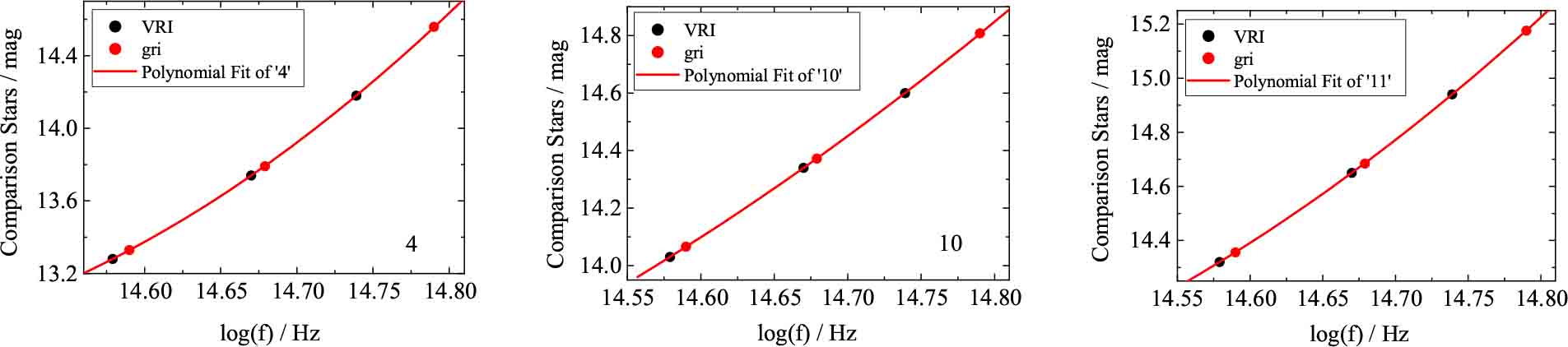
Fig. 1 For OJ 287, the gri fitting results of the three comparison stars.
Download figure:
Standard imageTable 1. Comparison Stars of OJ 287
| Star | V(error) | R(error) | I(error) | g | r | i |
|---|---|---|---|---|---|---|
| (1) | (2) | (3) | (4) | (5) | (6) | (7) |
| 4 | 14.18(0.04) | 13.74 (0.04) | 13.28 (0.04) | 14.56 | 13.79 | 13.33 |
| 10 | 14.60(0.05) | 14.34 (0.05) | 14.03 (0.05) | 14.81 | 14.37 | 14.07 |
| 11 | 14.94(0.04) | 14.65 (0.05) | 14.32 (0.05) | 15.18 | 14.68 | 14.36 |
Column (1): label of comparison stars; Col.(2): the magnitudes with error at V band; Col.(3): the magnitudes with error at R band; Col.(4) is the magnitudes with error at I band.
3. Optical variability
For OJ 287, we obtain 15094 gri observations in the 155 observational nights from 2014 December 13 to 2019 March 15. We use Ag = 0.093 mag, Ar = 0.064 mag, and Ai = 0.048 mag from NED (http://ned.ipac.caltech.edu/) to make the Galactic Extinction correction. The observations have been listed in Table 2.
Table 2. The Observations of OJ 287 at gri Band
| Date | JD | mg | σg | Date | JD | mr | σr | Date | JD | mi | σi |
|---|---|---|---|---|---|---|---|---|---|---|---|
| (+2457000) | (mag) | (mag) | (+2457000) | (mag) | (mag) | (+2457000) | (mag) | (mag) | |||
| (1) | (2) | (3) | (4) | (5) | (6) | (7) | (8) | (9) | (10) | (11) | (12) |
| 2014 – 12 – 13 | 5.312 | 14.829 | 0.045 | 2014 – 12 – 13 | 5.308 | 14.514 | 0.006 | 2015 – 3 – 21 | 103.082 | 14.097 | 0.009 |
| 2014 – 12 – 13 | 5.342 | 14.973 | 0.018 | 2014 – 12 – 13 | 5.312 | 14.504 | 0.009 | 2015 – 3 – 21 | 103.087 | 14.126 | 0.016 |
| 2014 – 12 – 13 | 5.346 | 14.970 | 0.018 | 2014 – 12 – 13 | 5.315 | 14.511 | 0.010 | 2015 – 3 – 21 | 103.090 | 14.108 | 0.017 |
| 2014 – 12 – 13 | 5.353 | 14.973 | 0.018 | 2014 – 12 – 13 | 5.319 | 14.507 | 0.010 | 2015 – 3 – 21 | 103.094 | 14.100 | 0.015 |
| 2014 – 12 – 13 | 5.356 | 14.967 | 0.018 | 2014 – 12 – 13 | 5.322 | 14.517 | 0.011 | 2015 – 3 – 21 | 103.097 | 14.121 | 0.005 |
| 2014 – 12 – 13 | 5.360 | 14.972 | 0.012 | 2014 – 12 – 13 | 5.326 | 14.509 | 0.015 | 2015 – 3 – 21 | 103.101 | 14.094 | 0.018 |
| 2014 – 12 – 13 | 5.363 | 14.985 | 0.022 | 2014 – 12 – 13 | 5.332 | 14.503 | 0.007 | 2015 – 3 – 21 | 103.104 | 14.105 | 0.014 |
| 2014 – 12 – 13 | 5.401 | 14.969 | 0.014 | 2014 – 12 – 13 | 5.335 | 14.504 | 0.004 | 2015 – 3 – 21 | 103.108 | 14.096 | 0.029 |
| 2015 – 3 – 21 | 103.082 | 15.149 | 0.007 | 2014 – 12 – 13 | 5.339 | 14.513 | 0.012 | 2015 – 3 – 21 | 103.111 | 14.073 | 0.008 |
| 2015 – 3 – 21 | 103.087 | 15.139 | 0.016 | 2014 – 12 – 13 | 5.342 | 14.510 | 0.009 | 2015 – 3 – 21 | 103.115 | 14.100 | 0.013 |
| 2015 – 3 – 21 | 103.090 | 15.171 | 0.025 | 2014 – 12 – 13 | 5.346 | 14.498 | 0.011 | 2015 – 3 – 21 | 103.118 | 14.110 | 0.010 |
| 2015 – 3 – 21 | 103.094 | 15.161 | 0.010 | 2014 – 12 – 13 | 5.353 | 14.505 | 0.012 | 2015 – 3 – 24 | 106.025 | 13.915 | 0.005 |
| 2015 – 3 – 21 | 103.097 | 15.145 | 0.023 | 2014 – 12 – 13 | 5.356 | 14.505 | 0.012 | 2015 – 3 – 24 | 106.037 | 13.908 | 0.018 |
| 2015 – 3 – 21 | 103.101 | 15.149 | 0.013 | 2014 – 12 – 13 | 5.360 | 14.500 | 0.008 | 2015 – 3 – 24 | 106.041 | 13.921 | 0.013 |
| 2015 – 3 – 21 | 103.104 | 15.158 | 0.027 | 2014 – 12 – 13 | 5.363 | 14.503 | 0.008 | 2015 – 3 – 24 | 106.045 | 13.942 | 0.005 |
| 2015 – 3 – 21 | 103.108 | 15.127 | 0.025 | 2014 – 12 – 13 | 5.367 | 14.506 | 0.007 | 2015 – 3 – 24 | 106.048 | 13.928 | 0.013 |
| 2015 – 3 – 21 | 103.111 | 15.133 | 0.025 | 2014 – 12 – 13 | 5.375 | 14.496 | 0.007 | 2015 – 3 – 24 | 106.052 | 13.924 | 0.021 |
| ... | ... | ... | ... | ... | ... | ... | ... | ... | ... | ... | ... |
| ... | ... | ... | ... | ... | ... | ... | ... | ... | ... | ... | ... |
| ... | ... | ... | ... | ... | ... | ... | ... | ... | ... | ... | ... |
Column (1): Date, at g band; Col.(2): JD(+2457000), at g band; Col.(3): g magnitude (mg ), in units of mag; Col.(4): uncertainty of mg (σg ), in units of mag; Col.(5): Date, at r band;k,./ Col.(6): JD(+2457000), at r band; Col.(7): r magnitude (mr ), in units of mag; Col.(8): uncertainty of mr (σr ), in units of mag; Col.(9): Date, at i band; Col.(10): JD(+2457000), at i band; Col.(11): i magnitude (mi ), in units of mag; Col.(12): uncertainty of mi (σi ), in units of mag. This table is available at http://www.raa-journal.org/docs/Supp/ms4807table2.pdf.
The g, r, i (gri) light curves are shown in Figure 2, in which, the upper panel stands for the g lightcurve, the middle panel stands for the r lightcurve, the lower panel stands for i lightcurve, and the red dots stand for the magnitude difference between two comparison stars '10' and '11'. There are six denser regions, which have been noted by the green rectangles, and noted as '1', '2', '3', '4', '5' and '6'.
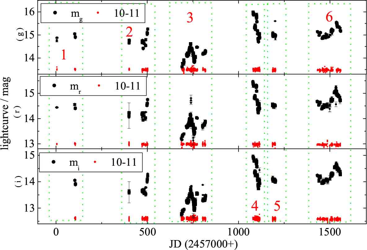
Fig. 2 The gri light curves of OJ 287. The upper panel stands for g-lightcurve, the middle panel stands for r-lightcurve, the lower panel stands for i-lightcurve. The red dots stand for the magnitude difference between two comparison stars '10' and '11'. There are six denser regions, which have been noted by the green rectangles.
Download figure:
Standard imageAt g band, there are 4900 observations, with the maximum variability Δ mg\max = 2.45 ± 0.03 mag from 13.57 ± 0.02 mag to 16.02 ± 0.03 mag. At r band, there are 5184 observations, with the maximum variability Δ mr |max = 2.35 ± 0.02 mag from 13.14 ± 0.02 mag to 15.49 ± 0.01 mag. At i band, there are 5010 observations, with the maximum variability is Δ mi|max = 2.36 ± 0.04 mag from 12.63 ± 0.03 mag to 14.99 ± 0.03 mag.
3.1. Intra-day Optical Variabilities
3.1.1. Methods
We use the following three methods to analyze the IDV results.
(1) The intra-day optical variabilities (IDVs) can be constrained as the following method. For any two pairs of observations (tj
, mj
, σj
), (tk
, mk
,σk
) (j, k = 1,2,...N), we calculated three parameters, time interval: Δ Tjk
= |tj
– tk
|, magnitude difference: Δ mjk
= |mj
– mk
|, and the standard deviation:  . If Δ mjk
> 3σjk
, we take Δ mjk
as a real variation and the corresponding time interval Δ Tjk
as the timescale. If there are more cases with Δ mjk
> 3σjk
, we take the shortest Δ Tjk
as the timescales as we did in our former papers (Fan et al. 2009a,b,c,2014).
. If Δ mjk
> 3σjk
, we take Δ mjk
as a real variation and the corresponding time interval Δ Tjk
as the timescale. If there are more cases with Δ mjk
> 3σjk
, we take the shortest Δ Tjk
as the timescales as we did in our former papers (Fan et al. 2009a,b,c,2014).
(2) The variability amplitude parameter (Heidt & Wagner 1996) (Am ),

here, mmax and mmin are the maximum and minimum magnitudes, and σmax and σmin are the corresponding uncertainties. When Am > 7.5%, the source is variable, and Δ T is the time scale.
(3) The variability parameter (Cj ), see Romero et al. (1999).
3.1.2. Results
We use the upper three methods to study the intra-day lightcurves, and use the Gaussian function to fit the regions of intra-day lightcurves when showing obvious variabilities. The intra-day variabilities are listed in Table 3. On one day, if there are more than one regions with intra-day variabilities, we list them in Table 4, and noted as, (1:GF), (2:GF), ...
Table 3. The IDV Analysis of OJ 287
| Band | Date | ΔT | Δm ± σ | Am | C | Date | ΔT | Δm ± σ | Am | C |
|---|---|---|---|---|---|---|---|---|---|---|
| (1) | (2) | (3) | (4) | (5) | (6) | (2) | (3) | (4) | (5) | (6) |
| g | 2016/3/26 | 95.90 | 0.11 ± 0.01 | 9.50 | 2.16 | 2017/12/10 | 183.02 | 0.22 ± 0.06 | 20.75 | 2.36 |
| (1:GF) | 95.91 | 0.11 ± 0.02 | (1:GF) | 44.08 | 0.09 ± 0.02 | |||||
| (2:GF) | 67.54 | 0.07 ± 0.02 | (2:GF) | 113.21 | 0.14 ± 0.03 | |||||
| 2016/12/18 | 248.11 | 0.08 ± 0.02 | 7.05 | 0.95 | (3:GF) | 64.77 | 0.17 ± 0.04 | |||
| (1:GF) | 81.07 | 0.06 ± 0.02 | 2017/12/11 | 142.13 | 0.14 ± 0.05 | 13.27 | 1.65 | |||
| (2:GF) | 49.52 | 0.06 ± 0.01 | (1:GF) | 7.69 | 0.06 ± 0.02 | |||||
| 2017/12/3 | 94.46 | 0.15 ± 0.03 | 13.45 | 1.55 | (2:GF) | 150.22 | 0.08 ± 0.02 | |||
| (1:GF) | 52.63 | 0.11 ± 0.03 | (3:GF) | 48.77 | 0.08 ± 0.00 | |||||
| (2:GF) | 74.30 | 0.11 ± 0.03 | (4:GF) | 77.36 | 0.11 ± 0.01 | |||||
| 2017/12/4 | 129.13 | 0.16 ± 0.03 | 14.29 | 1.71 | 2019/2/24 | 344.16 | 0.16 ± 0.04 | 15.49 | 1.27 | |
| 2017/12/9 | 135.94 | 0.15 ± 0.04 | 14.10 | 1.29 | (1:GF) | 101.23 | 0.07 ± 0.03 | |||
| (1:GF) | 28.54 | 0.06 ± 0.04 | (2:GF) | 65.30 | 0.05 ± 0.02 | |||||
| (2:GF) | 99.00 | 0.11 ± 0.03 | (3:GF) | 55.92 | 0.08 ± 0.03 | |||||
| (3:GF) | 49.84 | 0.09 ± 0.01 | 2019/3/16 | 33.70 | 0.08 ± 0.02 | 7.34 | 1.33 | |||
| (4:GF) | 54.00 | 0.10 ± 0.02 | (1:GF) | 26.93 | 0.08 ± 0.02 | |||||
| (2:GF) | 62.04 | 0.05 ± 0.01 | ||||||||
| r | 2017/11/26 | 148.46 | 0.13 ± 0.04 | 11.98 | 10.38 | 2017/12/11 | 155.52 | 0.10 ± 0.03 | 9.85 | 1.60 |
| 2017/12/3 | 114.77 | 0.11 ± 0.02 | 10.20 | 1.89 | 2019/2/20 | 371.09 | 0.26 ± 0.04 | 12.93 | 3.28 | |
| 2017/12/4 | 210.24 | 0.15 ± 0.04 | 13.87 | 5.81 | (1:GF) | 20.17 | 0.20 ± 0.04 | |||
| 2017/12/9 | 108.57 | 0.10 ± 0.03 | 9.56 | 1.56 | (2:GF) | 115.73 | 0.07 ± 0.03 | |||
| 2017/12/10 | 182.88 | 0.11 ± 0.02 | 10.02 | 1.69 | 2019/2/24 | 13.54 | 0.15 ± 0.04 | 13.96 | 2.43 | |
| (1:GF) | 33.70 | 0.06 ± 0.02 | 2019/3/16 | 155.23 | 0.08 ± 0.03 | 7.88 | 1.15 | |||
| (2:GF) | 40.81 | 0.11 ± 0.02 | (1:GF) | 27.07 | 0.07 ± 0.02 | |||||
| i | 2017/12/4 | 236.28 | 0.15 ± 0.05 | 15.76 | 1.88 | 2017/12/11 | 243.36 | 0.13 ± 0.02 | 12.13 | 1.30 |
| 2017/12/9 | 149.48 | 0.20 ± 0.05 | (1:GF) | 101.20 | 0.12 ± 0.03 | |||||
| 2017/12/10 | 203.18 | 0.20 ± 0.04 | 19.13 | 1.62 | (2:GF) | 20.35 | 0.11 ± 0.03 | |||
| (1:GF) | 74.97 | 0.09 ± 0.03 | 2017/12/26 | 256.32 | 0.11 ± 0.05 | 51.78 | 1.59 | |||
| (2:GF) | 47.23 | 0.12 ± 0.02 | (1:GF) | 115.20 | 0.10 ± 0.02 |
Column (1): Band; Col.(2): Date; Col.(3): the variable timescale, ΔT, in units of minutes; Col.(4): the variable value and the corresponding error, Δm ± σ, in units of mag; Col.(5): Am; Col.(6): C.
Table 4. Intra-day Periods of OJ 287
| Date | Band | PS | JUR | DCF | Po |
|---|---|---|---|---|---|
| (min) | (min) | (min) | (min) | ||
| (1) | (2) | (3) | (4) | (5) | (6) |
| 2017/12/10 | g | 94.97 ± 14.82 | 92.69 ± 9.65 | 93.69 ± 19.48, | 93.78 ± 3.66 |
| 212.21 ± 27.16 | |||||
| r | 103.5 ± 32.07 | 92.69 ± 7.43, | 88.2 ± 19.48, | 94.80 ± 12.32 | |
| 185.52 ± 8.46 | 189.16 ± 21.4 |
Column (1): Date; Col.(2): Band; Col.(3): PS, power spectrum results, in units of min; Col.(4): JUR, Jurkevich results, in units of min; Col.(5): DCF, DCF results, in units of min; Col.(6): Po , in units of min.
At g band, there are 9 days showing the IDVs, which are 2016/03/26, 2016/12/18, 2017/12/03, 2017/12/04, 2017/12/09, 2017/12/10, 2017/12/11, 2019/02/24 and 2019/03/16, see Figure 3 (the 1st, 2nd lines), with the variable timescales (Δ T) in the range from 7.69 min (Δ m = 0.06 ± 0.02 mag) to 344.16 min (Δ m = 0.16 ± 0.04 mag).
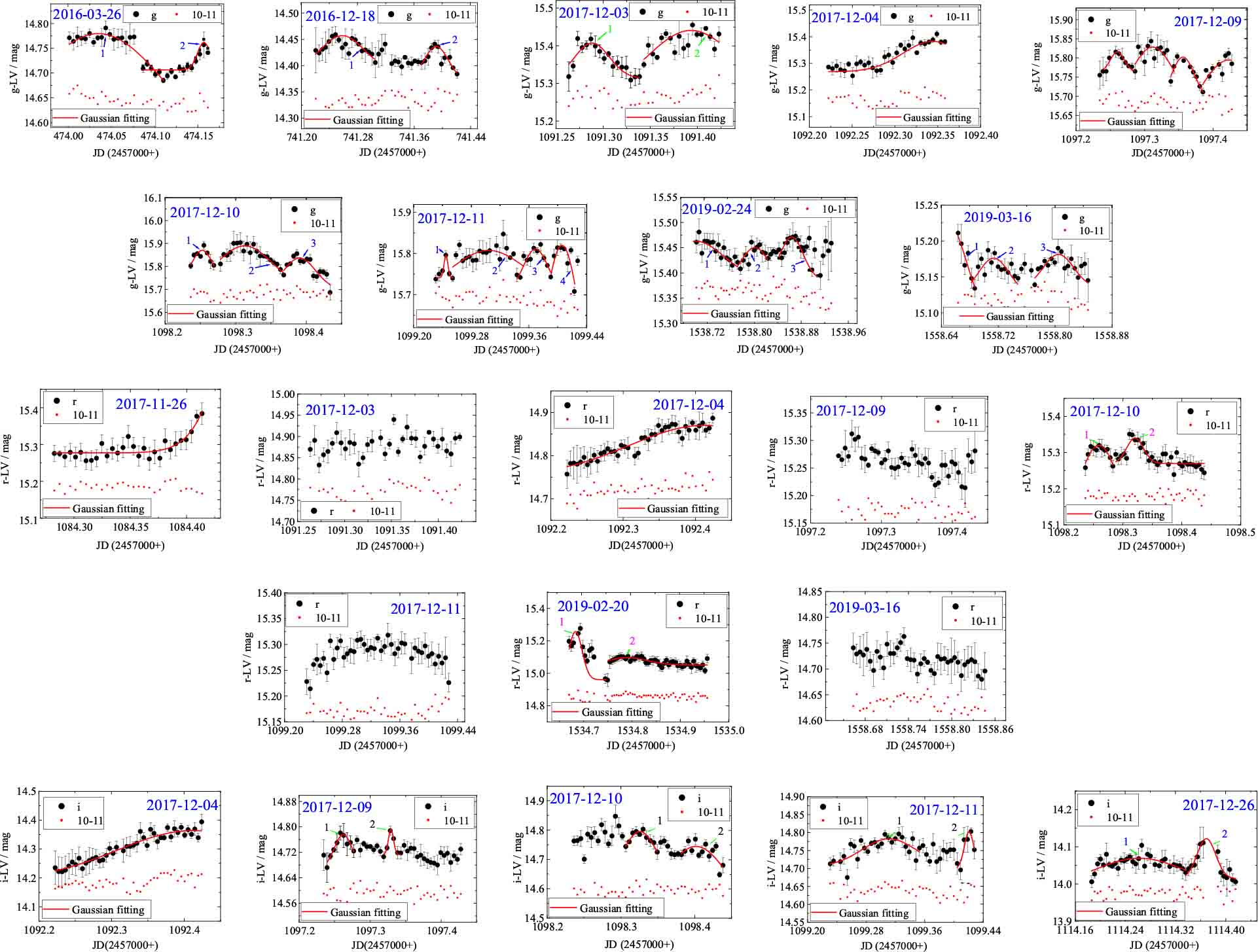
Fig. 3 The intra-day lightcurves of OJ 287 at gri bands, with the black dots standing for lightcurves, and the red lines being the Gaussian fitting.
Download figure:
Standard imageAt r band, there are 9 days showing the IDVs, which are 2017/11/26, 2017/12/03, 2017/12/04, 2017/12/09, 2017/12/10, 2017/12/11, 2019/02/20, 2019/02/24 and 2019/03/16 (the 3rd, 4th lines), see Figure 3, with the variable timescales (Δ T) in the range from 13.54 min (Δ m = 0.15 ± 0.04 mag) to 371.09 min (Δ m = 0.26 ± 0.04 mag).
At i band, there are 5 days showing the IDVs, which are 2017/12/04, 2017/12/09, 2017/12/10, 2017/12/11 and 2017/12/26 (the 5th lines), see Figure 3, with the variable timescales (Δ T) in the range from 20.35 min (Δ m = 0.11 ± 0.03 mag) to 243.36 min (Δ m = 0.13 ± 0.02 mag).
The relations between the gri variable timescales (ΔT) and variable values (Δm) are shown in Figure 4. At g band, Δ m = (3.05 ± 0.96) × 10−4Δ T + (0.07 ± 0.01), r = 0.51, p = 0.004, see the top-left panel in Figure 4; at r band, Δ m = (2.87 ± 0.91) × 10−4Δ T + (0.08 ± 0.01), r = 0.54, p = 0.04, see the top-right panel in Figure 4; at i band, Δ m = (1.42 ± 1.16) × 10−4Δ T + (0.10 ± 0.01), r = 0.40, p = 0.25, see the bottom-left panel in Figure 4. The correlation analysis imply that at g and r bands, Δ T and Δ m lie strong correlations; at i band, Δ T and Δ m lie no correlation.

Fig. 4 The relations between the gri variable timescales (ΔT) and variable values (Δm) of OJ287, with the red lines stand for linear fitting.
Download figure:
Standard imageFor all the data, Δ m = (2.91 ± 0.66) × 10−4Δ T + (0.08 ± 0.009), r = 0.52, p = 5.22 ± 10−5, see the bottom-right panel in Figure 4, which show that Δ m and Δ T have strong correlation.
3.2. Quasi-periodic Optical Variability
For blazars, it is difficult to judge the periodicity because of the uneven distribution of observations. To solve this problem, we can have two solutions. (1) By selecting appropriate fitting and interpolation methods, the non-uniform observations can be transformed into uniform data distribution. (2) We choose the appropriate method to deal with the non-uniform observations.
So we use the following process to deal with the periodicity of blazars. (1) Choose the suitable method to analyze the light curves with uneven observations and obtain the possible period (Po ). (2) Based on the regress analysis and interpolation to analyze the light curve, we obtain the uniform data distribution. (3) We obtain the periodicity (Pu ) of uniform data distributions. (4) Finally, we compare Po with Pu , and if Po is consistent with Pu , we choose Po as the period, otherwise, Po might be unreasonable.
3.2.1. Method
To deal with the uneven light curve, we use the power spectrum (PS), the discrete correlation function (DCF) and the Jurkevich method (JUR), to analyze the long-term optical variability, and choose the common part which can satisfy with each other in the error range as the possible period (Po ). Main introductions about the three methods can be seen in Fan et al. (2019).
3.2.2. Results
1. Intra-day periods
We use the three methods to calculate every intra-day lightcurves, with the main results in Table 4.
For OJ 287, there are possible periods on 2017 December 10 at g and r band. We use the Locfit Regression (Feigelson & Babu 2012) to fit the intra-day light curves and obtain the uniform data distributions, which can be analyzed by the upper three methods, and obtain the period of uniform data distributions (Pu ). The upper results are shown in Figure 5.
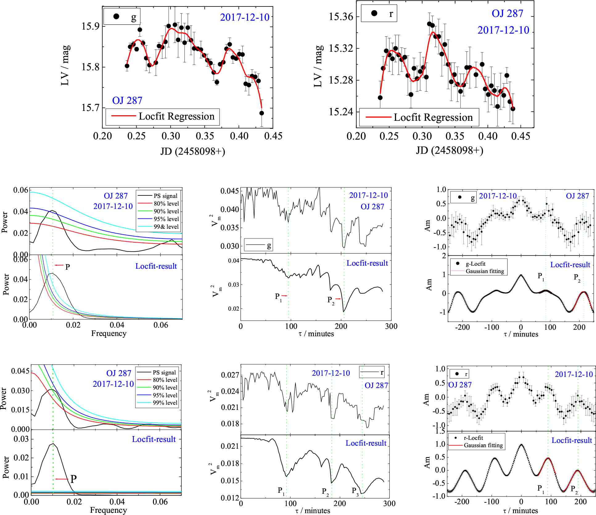
Fig. 5 The intra-day periods of OJ 287 at g and r band on 2017 December 10. The upper panels stand for intra-day light curves at g and r band, with red lines being the Locfit regression. The middle and lower panels stand for results calculated by the PW, JUR and DCF results respectively. In the PW results, the black, red, green, blue and cyan lines stand for power spectrum signals, the 80%, 90%, 95%, and 99% red noise levels respectively (Schulz & Mudelsee 2002).
Download figure:
Standard imageFor the results calculated by the three different methods, we choose the common parts which are consistent with each other within the error range as the period. From Figure 5, we can see that Po is consistent with Pu , which are noted by the red dotted lines, so we choose Po as the period, at g band, Pg = 91.99 ± 5.66 min, at r band, Pr = 93.30 ± 3.15 min. The periods from two different bands are consistent with each other, which imply that the physical origins of g and r emissions are correlated.
2. Long-term periods
To analyze the long-term variability more comprehensively, we combine our observations with the available data from the literature (Pollock et al. 1971; Schaefer et al. 1980; Lloyd 1984; Sillanpää et al. 1988; Jia et al. 1995; Soltan et al. 1996; Jia et al. 1998; Xie et al. 1988; Bai et al. 1999; Ghosh et al. 2000; Wu et al. 2006; Zheng et al. 2008; Villforth et al. 2010; Dai et al. 2011; Pihajoki et al. 2013; Rakshit et al. 2017), and SMARTs (the Small and Moderate Aperture Research Telescope System).
We combine the whole available data in Figure 6 (the upper panel), in which, the black dots stand for the data from the literature, and the red dots stand for our observations.

Fig. 6 Long-term optical lightcurves and periodic analyses of OJ 287. The upper panel stands for the long-term lightcurves, with the blue dots from this work, and the red line being the Locfit regression. The middle and lower panels stand for results calculated by the power spectrum, Jurkevich results, and the DCF results respectively.
Download figure:
Standard imageBased on power spectrum, the results are Pp = 0.48 ± 0.05, 1.91 ± 0.05, 12.02 ± 0.41 and 18.35 ± 0.48 yr; based on Jurkevich method, the results are PJ = 1.31 ± 0.27, 3.93 ± 0.13, 5.90 ± 0.53, 11.93 ± 0.4 and 22.96 ± 0.55 yr; based on DCF method, the results are PD = 12.13 ± 1.82, 24.25 ± 2.28 and 37.04 ± 1.8 yr. We choose the common parts, and obtain the suspected period Po = 12.02 ± 0.41 yr.
We use the Locfit Regression (Feigelson & Babu 2012) to fit the long-term light curves and show the results in Figure 6 (red line in the upper panel). After calculation, the possible period is Pu = 12.80 ± 0.95 r, which is consistent with Po , so period of OJ 287 might be P = 12.02 ± 0.41 yr.
3.3. Relations between Flux Densities and Spectral Indices
3.3.1. Methods
To obtain the optical spectral index (α), firstly, we convert the magnitude (mν ) into flux density (Fν ); then, we use the relation Fν ∝ ν−α to calculate the spectral index (α), here ν is frequency (ν = g, r and i).
We use the linear fitting to analyze the relations between the spectral indices (α) and flux densities (Fν ) (ν = g, r, i): Fν = k × α + b. In this process, p is the chance probability of linear fitting, and r is the correlation coefficient.
To analyze the spectral behaviors when source is in the different state of the source's brightness, we study the Fν – α correlations based on the fixed flux interval (Fν|i ), and use the slope ki to compare the correlations, here i = 1,2,...,n, n is the total number of flux interval.
3.3.2. Results
After calculation, there are 4639 spectral indices (α), which are in the range from 0.39 ± 0.02 to 1.24 ± 0.02, with the averaged value  .
.
At g band, α = –(1.91 ± 0.05) × 10−2 Fg + (0.87 ± 0.003), with r = –0.50, p = 1.49 × 10⁻⁴, see Figure 7 (the left panel).
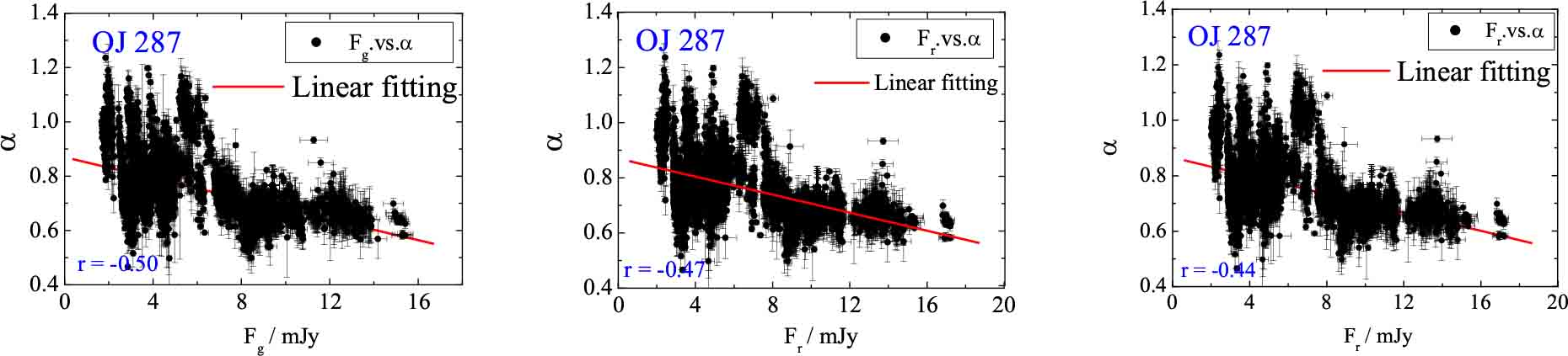
Fig. 7 The relations between the spectral indices (α) and flux densities (Fgri ) of OJ 287, with the red lines stand for linear fitting.
Download figure:
Standard imageAt r band, α = –(1.67 ± 0.05) × 10−2 Fr + (0.87 ± 0.003), with r = –0.47, p = 7.55 × 10⁻⁵, see Figure 7 (the middle panel).
At i band, α = –(1.25 ± 0.04) × 10−2 Fi + (0.86 ± 0.003), with r = –0.44, p = 1.37 × 10⁻⁵, see Figure 7 (the right panel).
4. Discussion
4.1. Optical Variability
For OJ 287, Fan et al. (2009a) obtained the IDVs with the timescales in the range from 10 min to 2 hour with the variations from 0.11 mag to 0.75 mag. Gaur et al. (2012) found evident intra-day variabilities. In this work, we obtain that, at g band, the variable timescales are in the range of 7.69∼344.16 min; at r band, the variable timescales are in the range of 13.54∼210.24 min; at i band, the variable timescales are in the range of 6.62∼276.77 min.
Some works claim to find the intra-day periods, but have not been confirmed (e.g., Frohlich 1973; Visvanathan & Elliot 1973; De Diego & Kidger 1990). For example, Visvanathan & Elliot (1973) obtained a period of ∼40min at optical band for OJ 287.
In this work, for OJ 287, we obtain the consistent periods at g and i bands on 2017 September 10. OJ 287 is famous for the discovery of the convincing period about 12 yr (Sillanpää et al. 1988). Many models have been proposed to explain this period, which can be classed into two types: dynamical models and geometrical models (Liu & Wu 2002; Kushwaha 2020). The dynamical models show that the period is caused by the accretion dynamics in the supermassive binary black holes (SBBHs) (Sillanpää et al. 1988; Lehto & Valtonen 1996; Valtonen et al. 2008), while the geometrical models consider that the period caused by the Doppler boosted jet emission from the jet procession (Katz 1997; Villata et al. 1998; Britzen et al. 2018; Qian 2018).
Goyal et al. (2018) analyzed the long-term optical light-curves (∼117 yr), but did not find the period of 12 yr. In this work, based on our observations and the data from the available literature, we analyze the long-term lightcurves and obtain the period P = 12.02 ± 0.41 yr, which is consistent with that of Lehto & Valtonen (1996)'s.
For this source, we find that there are strong correlations between the IDV timescales (Δ T) and the corresponding variable values (Δ m). Based on the results from Fan et al. (2009b), we can obtain Δm = (–0.002 ± 0.001) Δ T + (0.44 ± 0.07), with r = –0.40, p = 0.11, which is different from the result in this work, seeing Figure 8.
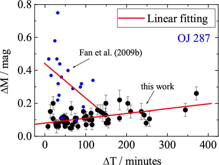
Fig. 8 The relations between the IDV timescales (Δ T) and variations (Δ m). The black dots stand for the data from this work, and the blue dots from Fan et al. (2009b).
Download figure:
Standard image4.2. Mass of the Central Black Hole
The origin of IDV timescales might come from the inner part of the blazar, and they are close to the black hole. In this sense, the IDV timescale can be used to estimate the mass (Abramowicz & Nobili 1982). For this source, we obtain the intra-day period P ≈ 95 min.
Based on the expression from Fan et al. (2014), the emission regions can be calculated as follows.
(1)  (thin accretion disk with Schwarzschild black hole);
(2)  (thick accretion disk with Schwarzschild black hole);
(3)  (Kerr black hole, with the radius of the event horizon r, angular momentum parameter a).
If we take the period, P as the time for the light travel in the innermost stable orbit, then 2 π r = c P/(1 + z), so the black hole mass should be
(1)  (thin accretion disk with Schwarzschild black hole);
(2)  (thick accretion disk with Schwarzschild black hole);
(3)  (Kerr black hole, with the radius of the event horizon r, angular momentum parameter a).
We use the upper method to obtain the lower limit of central black hole mass. For OJ 287, z = 0.3056, and P ≈ 95 min, so the corresponding masses of the black holes should be more than 2.31 ∼ 14.04 (× 107 M⊙). Cao (2003) pointed out the black hole mass of OJ 287 less than 6.16 × 10⁸ M⊙, which is consistent with our result. Gupta et al. (2017) used the variable timescale to obtain the mass 6.5 ∼ 16.7(× 107 M⊙), which is very close to ours.
4.3. Binary Black Hole System
Considering the binary black hole system, with the semi-major axes being b1 and b2, the value of b1 + b2 can be calculated by the Kepler's law,
which can be transformed as:

here, M8 and m8 are masses of the primary and secondary black hole, in units of 108 M⊙, P is period, G is the gravitational constant, r16 = a1 + a2, in units of 1016 cm.
Based on the work of Sillanpää et al. (1988), r ∼ 0.1 pc. In this work, P = 12.02 yr, the secondary black hole mass m8 = 0.231 ∼ 1.404. Based on Equation (2), we can obtain the primary black hole mass M8 ≈ 74, that is, M = 7.4 × 10⁹
M⊙, which is close to the value 1.8 × 10¹⁰
M⊙ calculated from Valtonen et al. (2012). Sillanpää et al. (1988) give the ratio  is 0.004, our value is about 0.003 ∼ 0.019. The SMBH estimated by the IDV timescales gives a lower limit, so that mass is smaller than the mass estimated here.
4.4. The Relations between the Flux Densities and Spectral Indices
For OJ 287, our results show the BWB behaviors at g, r and i bands. Dai et al. (2011) used the observations during an optical outburst to find a BWB chromatism. Bonning et al. (2012) found the BWB behaviors, as well as the redder-when-brighter (RWB) behaviors. Siejkowski & Wierzcholska (2017) did not reveal any BWB or RWB behaviors whenever the source was in any state of activity. Soltan et al. (1996) found that the color indices were stable during the outburst in 1993–1994.
To study the difference of the relations between Fν and α when the source is in the different state of brightness, we divide the Fν -α distributions into some sub-distributions according to the fixed flux span (Fν|0), which can be calculated by the Jurkevich method from the Fν -α distributions. Then, we calculate the correlations between Fν and α from every sub-distribution.
For OJ 287, Fg|0 = 1.16 mJy, Fr|0 = 1.38 mJy, Fi|0 = 1.98 mJy, which have been placed in the top right corner of Figure 9. The correlations between Fν and α from every sub-distribution have been noted in Figure 9, in which the red lines stand for the linear fitting. Most of the sub-distributions show BWB, especially when the source is in the state of brightness.
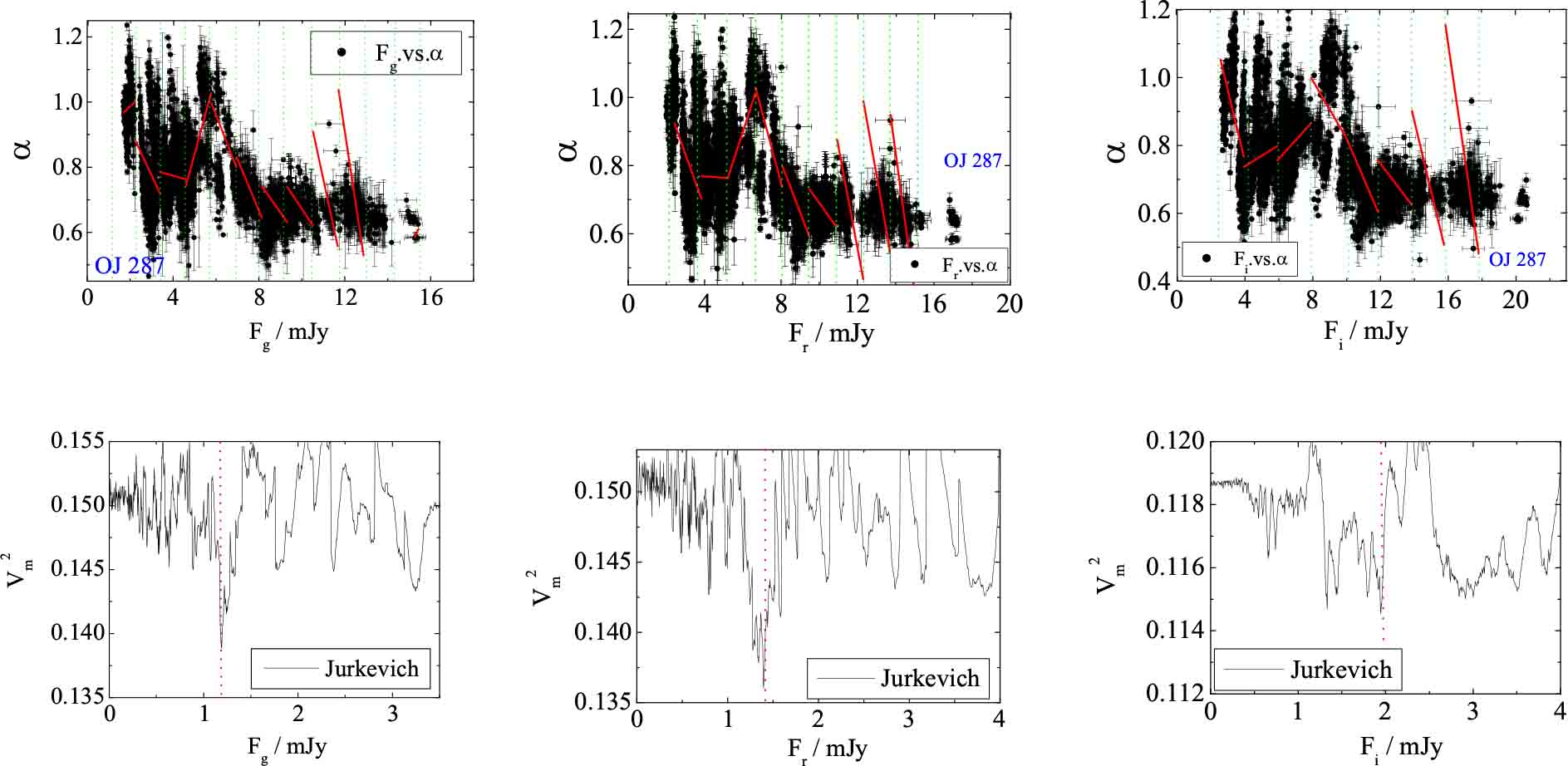
Fig. 9 For OJ 287, the correlations between Fν and α in the sub-distributions limited by a fixed flux span (Fν|0). The lower three panels stand for the analyzed results based on different span using the Jurkevich method.
Download figure:
Standard image4.5. Time Delay among Different Bands
We use the DCF method to analyze the time delays among the gri lightcurves and we plot the results in Figure 10. For the gross lightcurves, we cannot find time delay among gri bands, see Figure 10 (the first line), and find sub-structures, which are noted by 'a' and 'b', and might come from the different stages of the lightcurves.

Fig. 10 The time delays among different bands for OJ 287. The upper row of three panels stand for the results calculated from the gross lightcurves, the other four rows of panels stand for the results calculated from the part regions, with the red lines stand for the Gaussian fitting.
Download figure:
Standard imageThe lightcurves of OJ287 can be divided into six denser stages, which are noted as '1', '2', '3', '4', '5' and '6', see the green dotted rectangles in Figure 2. We analyze the time delays from different stages, and plot the results in the lower four lines of Figure 10. In some stages ('2', '3', '4' and '5'), there are time delays, but the delay time is different, for example, τri|2 = 12.14 ± 1.88 min, τri|3 = 8.03 ± 3.77 min, τri|45 = –11.46 ± 6.66 min; in stage '6', no time delay.
5. Conclusions
In this work, we present the gri photometric results of the BL Lac objects OJ 287, which are obtained using the 1.26m telescope at the Xinglong Observatory. Based on these observations, we obtain the following conclusions.
1. During our monitored duration, we find two types of intra-day variabilities (IDVs), non-periodic IDVs and periodic IDVs. In no periodic IDVs, the variable timescales (Δ T) and variable values (Δ m) have strong correlations. The causes of two types of IDVs are not clear or definite. To identify the causes, further observations and improvement of the emission theory are required.
2. We analyze the long-term lightcurve of OJ 287, and obtain the likely period P = 12.02 ± 0.41 yr. Based on that period and the binary black hole model, we obtain the mass ratio ( ) between the primary and secondary black hole is 0.007, which is very close to the others.
3. For OJ 287, the relations between Fν and α show BWB behaviors, even if this source is in a different state of the source's activity.
Acknowledgements
The work is partially supported by the National Natural Science Foundation of China (Grant Nos. U1831119, U1531245, U1431112, 11733006, 11503004 and 11403006), Science and Technology Program of Guangzhou (201707010401). This research has made use of SMARTS optical/near-infrared light curves that are available at www.astro.yale.edu/smarts/glast/home.php.