Abstract
We simulate the evolution of supernova remnants (SNRs) in a strong magnetic field. Usually, supernovae explode in a normal interstellar medium with magnetic field of no more than 50 μG, which has been well studied. However, the surrounding magnetic field will be much stronger in some situations, such as in a galactic center. Therefore, we try to explore these situations. The simulations show that a strong magnetic field of 1 mG will align the motion of ejecta in a way similar to a jet. The ejecta propagating perpendicularly to the magnetic field will be reflected and generate a strong reverse shock. When the reverse shock converges in the explosion center, it will more or less flow along the central magnetic field. Finally, most of the ejecta will propagate parallel to the magnetic field.
Export citation and abstract BibTeX RIS
1. Introduction
Supernova remnants (SNRs) can accelerate cosmic rays and are taken as important targets for interstellar medium (ISM) research (Morlino & Caprioli 2012; Bell et al. 2013; Zhu et al. 2014; Jogler & Funk 2016). To study their evolution, numerical simulation is an effective method, but it is difficult to estimate the initial conditions used in simulations. Usually, we just set canonical values for some uncertain parameters, so some special situations will be ignored. For example, in themagnetohydrodynamics (MHD) of SNRs, the initial magnetic field is almost impossible to calculate directly, so it is always set to a reasonable value in most related works (Orlando et al. 2007; Schneiter et al. 2010; Fang & Zhang 2012; Zhang et al. 2017, 2018). As a result, we never simulate the evolution of SNRs in a very strong magnetic field.
Although the canonical interstellar magnetic field in the Milky Way is about 10 μG (Crutcher 2012; Haverkorn 2015), it is possible for the magnetic field to reach 1 mG in dense interstellar clouds (Ferriére 2009) and 100 mG in some maser regions. The maser regions are usually so small that they cannot influence the evolution of SNRs, but there are many large dense clouds in a galactic center, and they also exist to a greater or lesser extent in a galactic disk or a star cluster. Therefore, we can imagine an SNR evolving in a strong magnetic field. However, nobody has ever tried to simulate this situation, because we have not actually observed such magnetic fields in SNRs, so it will be interesting to explore such a situation. In fact, similar situations have been studied in many research efforts (Balsara & Spicer 1999; Stone & Gardiner 2009; Barnes et al. 2018), but these works pay more attention to testing a new algorithm or scheme. Although they simulate a blast in a relatively strong magnetic field, the parameters they used are completely different from an SNR. As a result, these results possibly show similar images to SNRs, but the physics is different.
In this paper we report our discovery from such an MHD simulation. Meanwhile, we also simulate an SNR in a normal magnetic field as a comparison. In Section 2, we describe the simulation model and list the parameters we use. In Section 3, we present and discuss the results. Section 4 is a summary.
2. Model
We use a 3D MHD frame with a grid of 128 × 128 × 128 and a resolution of 0.47 pc pixel−1. Moreover, we perform adaptive mesh refinement (AMR) simulation and calculate the ratio (β) of the thermal pressure to the magnetic pressure in some important images. In the simulation, we ignore the cooling effect which is possibly important in old SNRs. The evolution of an SNR is divided into three phases, the ejecta-dominated (ED) phase, the Sedov-Taylor (ST) phase and the pressure-driven snowplow (PDS) phase (Truelove & McKee 1999). During the ED phase, the ejecta is dynamically much more important than in the ST phase. The ED phase has been studied well, because we can focus on the ejecta to study the evolution and ignore some complex factors, such as the ISM density distribution and the magnetic field. The first two phases are classified as "nonradiative," but the radiative loss becomes important in the PDS phase. The cooling effect will become important gradually during the evolution of an SNR, but it is not a dominant factor before 10 000 years, the time duration used for this simulation. The simulation is based on the set of ideal conservation equations
in which ρ is mass density, v is velocity, B is magnetic field intensity, P* is total pressure and E is total energy density.
For a 20 M⊙ star, the ejecta mass is about 15.8 M⊙ (Sukhbold et al. 2016) and the explosion kinetic energy is about 2.0 × 1051 erg (Poznanski 2013; Müller et al. 2016). In total, we perform three simulations with different magnetic field intensity (B) and surrounding ISM density (n). At first, we simulate a typical SNR in a normal environment with B ∼ 9 μG and n ∼ 0.5 cm−3. The second set is B∼900 μG and n∼0.5 cm−3, while the third is B∼900 μG and n∼10 cm−3, an environment more similar to a molecular cloud. Because a dense cloud is possibly not so large that it can cover the whole evolution of an SNR, we simulate two situations. To reach the ST phase, it will take 693 and 1881 years respectively for n∼10 and 0.5 cm−3 (Leahy & Williams 2017). In order to simulate a spherically symmetric explosion, we set an initial radius of 4 pc, before which we just use the result calculated based on Leahy & Williams (2017). In other words, we place the initial ejecta, i.e., the supernova, within 4 pc. We can estimate the velocity, density and pressure in this region by running a program written by Leahy & Williams (2017). This program optimizes the analytical solution suggested in Truelove & McKee (1999) and provides many convenient functions.
Table 1. Summary of Simulation Parameters
| Parameters | Values | References |
|---|---|---|
| SNR Parameters | ||
| Initial Mass | 20 M⊙ | |
| Ejecta Mass | 15.8 M⊙ | [ |
| Explosion Kinetic Energy | 2.0 × 1051 erg | [ |
| Initial Radius | 4 pc | |
| Initial Time | 693 and 1881 yr | [ |
| Total Time | 10 000 yr | |
| Other Parameters | ||
| Mean Number Density (n) | 0.5 and 10 cm−3 | [ |
| Magnetic Field Intensity (B) | 9 and 900 μG | [ |
| Mean Atomic Weight | 1.3 | |
| Adiabatic Coefficient | 1.7 | |
[1]Sukhbold et al. (2016) [2]Poznanski (2013) [3]Müller et al. (2016) [4]Leahy & Williams (2017) [5]Nakanishi & Sofue (2006) [6]Nakanishi & Sofue (2016) [7]Haverkorn (2015) [8]Ferrière (2009).
The simulation is performed by PLUTO1 (Mignone et al. 2007, 2012). We summarize the parameters in Table 1, and list the references below. The parameters are not entirely the same as the references, because we adjust some values according to our scientific targets.
3. Results and Discussion
We display the simulation for an SNR in a normal environment in Figure 1. It is obvious that the shock wave plows the ISM and leaves a low density and weak magnetic field in the center. Compression of the magnetic field is different in different directions. The two edges parallel to the magnetic field show higher density and stronger magnetic field. If we observe it in radio waveband, the two edgeswill be brighter and form a bilateral SNR. In addition, with the evolution of the SNR, we can see some material flow toward the interior, i.e., the reverse shock. The reverse shock is fast, but will not carry lots of material. As a result, the center of the SNR is still low-density.
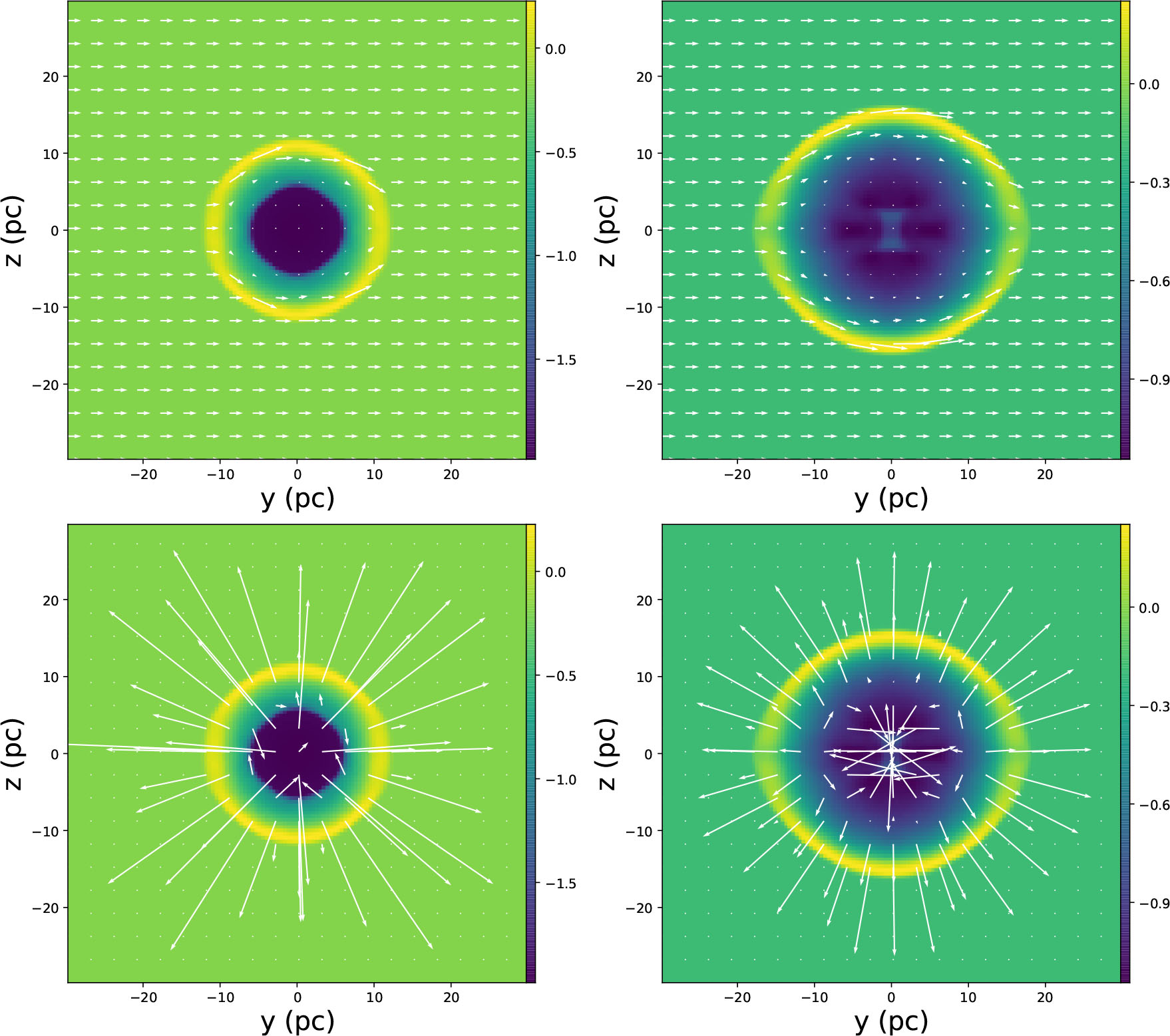
Fig. 1 Simulation for a normal environment in the disk of the Milky Way. The colored patterns indicate the density distribution with units of log(cm−3). The white arrows indicate the magnetic field and velocity respectively in the top and bottom two panels. The left and right panels respectively show the results after 4500 and 10 000 years. We should add 693 years to this time if we want to obtain the age.
Download figure:
Standard imageHowever, it becomes completely different in a strong magnetic field (Fig. 2). In the center of the SNR, the magnetic field becomes weak at the beginning, but finally recovers, because the magnetic field is strong and the ejecta cannot influence it for a long time. We can only see a little compression of the magnetic field, and the two edges perpendicular to the magnetic field are much denser, which can cause brighter radio emission where the magnetic field is perpendicular to the shock surface. From the velocity images, we can find the reason. The strong magnetic field will reflect the ejecta and form a denser and lasting reverse shock, which enriches the two edges propagating along the magnetic field. This is interesting, because most SNRs exhibit bright shells where the magnetic field is perpendicular to the shock surface, similar to the first simulation we did. However, there is actually a special case, SN 1006, whose magnetic field is perpendicular to the shock surface (Reynoso et al. 2013). This is explained by a quasi-parallel model (Schneiter et al. 2015), but is still unsolved currently (Petruk et al. 2009). Of course, our simulation cannot be used to explain it, because its magnetic field is very weak. However, our simulation implies there is possibly an unknown mechanism collimating the ejecta from SN 1006.

Fig. 2 Simulation for an environment with B∼900 μG and n∼0.5 cm−3. The colored patterns represent the density distribution with units of log(cm−3). The white arrows represent the magnetic field and velocity respectively in the top and bottom six images which show the results after 1500, 2500, 3500, 4500, 7500 and 10 000 years. We should add 693 years to this time if we want to obtain the age.
Download figure:
Standard imageTo study the formation of reverse shock in the shock region, we execute the AMR simulation for the early evolution and plot β maps (Fig. 3). We apply four levels in the AMR simulation and show the boxes to illustrate the AMR configuration, but delete boxes in the last image to make the pattern clear. The β maps fluctuate greatly, so we use log scale in the maps at 2500, 3500 and 4500 years. The evolution tendency is similar to low-resolution simulation, but some details are different. In denser regions, two shells appear, possibly also caused by reverse shock. The reverse shocks propagating along the y-axis are possibly much stronger than those along the z-axis, so they converge in the center and push those along the z-axis to form two shells. However, the initial surrounding density is uniform, so this can only originate from the difference in magnetic field. In β maps, we find the magnetic pressure is even higher than the thermal pressure, which indicates that the magnetic pressure strengthens the reverse shock along the z-axis. This is more evidence supporting our explanation for the formation of denser regions.

Fig. 3 AMR simulation and β map for an environment with B∼900 μG and n∼0.5 cm−3. The top four images show the AMR simulation density distribution with units of cm−3 after 1500, 2500, 3500 and 4500 years. The bottom four images (continued on the next page) display the β map after 1500, 2500, 3500 and 4500 years, in which the first image uses a dimensionless unit and the other three images use a log unit. We should add 693 years to this time if we want to obtain the age.
Download figure:
Standard imageActually, similar patterns in other studies (Balsara & Spicer 1999; Stone & Gardiner 2009; Barnes et al. 2018) originate from a similar mechanism, but we specify this for SNRs and use relatively higher resolution. Moreover, Parrish & Stone (2007) also notice the plasma will propagate along magnetic field lines and study magnetothermal instability in such a system. We do not find obvious magnetothermal instability in our simulation, because we use different parameters.
We also simulate an SNR evolving in a dense cloud all the time (Fig. 4). The result is similar to the second one, but it evolves much more slowly. It manifests two dense edges and two low-density edges, which hint at a difference in the radio and X-ray images, if we believe the radiation of such an SNR totally originates from a synchrotron mechanism. The synchrotron radiation spectrum will have a cutoff at the X-ray waveband, so the power-law spectrum will have two or more spectral indices. As a result, the radio and X-ray fluxes are not always proportional to each other. Sometimes, a region with higher magnetic field and lower density is brighter at the X-ray waveband than a region with lower magnetic field and higher density. In contrast, a region with higher magnetic field and lower density is fainter at radio waveband. This will possibly cause the X-ray and radio patterns of an SNR to not overlap, just like SNR G1.9+0.3 (Reynolds et al. 2008; Borkowski et al. 2017). Nevertheless, SNR G1.9+0.3 is the youngest SNR in the MilkyWay and the parameters we used in the simulation are not very consistent with it. Therefore, we cannot currently assert the origin of peculiar X-ray/radio patterns in this SNR.
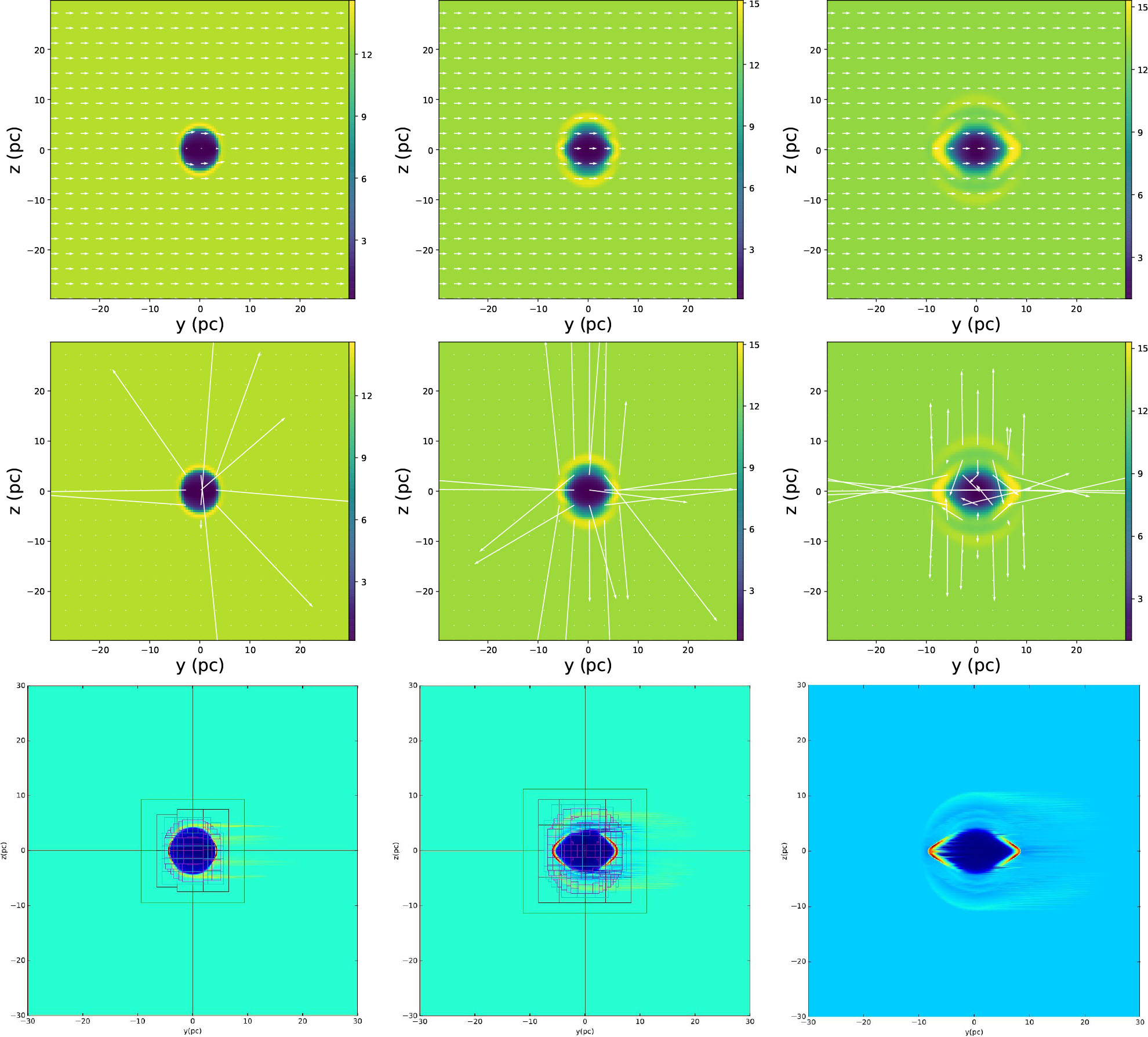
Fig. 4 Simulation for an environment with B∼900 μG and n∼10 cm−3. The colored patterns indicate the density distribution with units of cm−3. The white arrows represent the magnetic field and velocity respectively in the top and middle three images which display the results after 1500, 4500 and 10 000 years from left to right respectively. The bottom three images depict the AMR results. We should add 1881 years to this time if we want to obtain the real age.
Download figure:
Standard imageIn addition, the high-resolution image at 10 000 years shows three shells along the z-axis on one side. This is similar to the phenomenon in the aforementioned simulation with n∼0.5 cm−3, but the direction is reversed. The difference between the two phenomena is only the surrounding density and evolution time. They should both originate from reverse shock, but we cannot find a perfect explanation for this based on the present simulation. Moreover, Zhang et al. (2018) try to study the radio morphology of SNRs and successfully explain five types of SNR, but multi-layer and irregular SNRs are still puzzling. In our view, these phenomena can help us understand the formation of multi-layer SNRs.
4. Summary
We simulate the evolution of SNRs in a normal environment, a galactic center and a large dense cloud. Here we summarize the conclusions as follows:
- In a strong magnetic field, the edges compressed by the SNR are different from those in a weak magnetic field because of plowing by the reverse shock.
- A strong magnetic field will align the propagating direction of ejecta from an SNR, which will lead to a phenomenon similar to a jet.
- An SNR evolving in a strong magnetic field will possibly show strange radio and X-ray patterns.
To further study these results, more observations and large-scale high-resolution simulations are necessary. In addition, our work provides us a clue on how to solve the puzzle of SNR G1.9+0.3 and multi-layer SNRs, but we need more detailed simulations to confirm this.
Acknowledgements
This work is supported by the National Key R&D Program of China (2018YFA0404203).