

Abstract
We introduce a 0.7 m telescope system at the Miryang Arirang Astronomical Observatory (MAAO), a public observatory in Miryang, Korea. System integration and a scheduling program enable the 0.7 m telescope system to operate completely robotically during nighttime, eliminating the need for human intervention. Using the 0.7 m telescope system, we obtain atmospheric extinction coefficients and the zero-point magnitudes by observing standard stars. As a result, we find that atmospheric extinctions are moderate but they can sometimes increase depending on the weather conditions. The measured 5σ limiting magnitudes reach down to BVRI = 19.4–19.6 AB mag for a point source with a total integrated time of 10 minutes under clear weather conditions, demonstrating comparable performance with other observational facilities operating under similar specifications and sky conditions. We expect that the newly established MAAO 0.7 m telescope system will contribute significantly to the observational studies of astronomy. Particularly, with its capability for robotic observations, this system, although its primary duty is for public viewing, can be extensively used for the time-series observation of transients.
Export citation and abstract BibTeX RIS

Original content from this work may be used under the terms of the Creative Commons Attribution 3.0 licence. Any further distribution of this work must maintain attribution to the author(s) and the title of the work, journal citation and DOI.
1. Introduction
The role of small telescopes with an aperture size of ≲1 m is still crucial in modern time-domain astrophysics. With the advantages of a wide field of view (FOV), low price, and easy accessibility, small telescopes remarkably increased the number of discoveries and the light curves of transients (e.g., classical novae, supernovae (SNe), luminous blue variables, etc.) in various surveys such as the Palomar Transient Factory (Law et al. 2009), the Catalina Real-Time Transient Survey (Drake et al. 2009), the All-Sky Automated Survey for Supernovae (Shappee et al. 2014), the Asteroid Terrestrial-impact Last Alert System (Tonry et al. 2018), the Zwicky Transient Facility (Bellm et al. 2019; Graham et al. 2019), the Korea Microlensing Telescope Network (Kim et al. 2016), and the Intensive Monitoring Survey of Nearby Galaxies (Im et al. 2019).
Recently, transients at short timescales (e.g., less than a few days), referred to as fast transients have been detected. Fast transients includes SNe early light curves (Hosseinzadeh et al. 2017, 2022; Ni et al. 2022; Lim et al. 2023), M-dwarf flares (Schmidt et al. 2019; Rodríguez Martínez et al. 2020), optical afterglow of gamma-ray bursts (Piran 2004; Dichiara et al. 2022; Kumar et al. 2022), and kilonovae (Lyman et al. 2018; Jin et al. 2020). These fast transients allow us to understand their progenitor systems, explosion mechanisms, and interactions with their ambient environment, making the observation of fast transients important. However, due to short duration time of fast transients (e.g., ∼a sub-hour to days; Andreoni et al. 2020; Strausbaugh et al. 2022), many aspects of their nature remain uncovered.
To successfully detect these fast transients, observations should be performed immediately when the transients occur, using a system that operates without human intervention, known as robotic observation. Robotic telescopes can perform scheduled observations based on the programmed observing plans, which reduces costs and uses nighttime fully. It is not a surprise that many small telescopes have already been operated robotically (Hardy et al. 2015; Im et al. 2015; Kasper et al. 2016; Bellm et al. 2019; Law et al. 2022). These telescopes can respond fast to transient alerts, giving us the chance to perform imaging and spectroscopic follow-up observations using other telescope networks (e.g., Im et al. 2021).
The 0.7 m telescope system was installed in 2020 May in the 7.7 m diameter round dome at MAAO in Miryang, Korea (35°30 08
08 6N, 128°45400E, 95 m). While MAAO primarily serves as a science museum for public education, it can also function as an astronomical research facility.
This paper is organized as follows. We present the characteristics of the system in Section 2. In Section 3, we describe the schematic of the system integration and the process of the robotic observation based on the scheduler. The system performances, such as point-spread function (PSF) shape variation, standard flux calibration, and limiting magnitudes, are presented in Section 4. Sections 5 and 6 discusses current research topics and future prospects, and in Section 7, a summary is provided. In this work, all magnitudes are in the AB system unless otherwise specified.
2. System Characteristics
2.1. Telescope and Mount
The optical system of the 0.7 m telescope is designed as a Corrected Dall-Kirkham system (CDK700) with a focal ratio of 6.5, which is produced by PlaneWave Instruments. It consists of three main components: an ellipsoidal primary mirror (700 mm in diameter), a spherical secondary mirror (312.4 mm in diameter), and an additional lens group to prevent image distortions such as coma, off-axis astigmatism, and field curvature. Both mirrors are made from fused silica, a material known for its excellent optical properties. Figure 1 shows the telescope mounted on an alt-azimuth mount system and equipped with dual Nasmyth foci, allowing for visual and CCD observations.
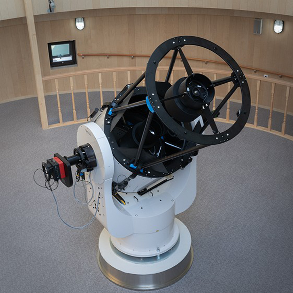
Figure 1. The 0.7 m telescope at MAAO.
Download figure:
Standard image High-resolution imageFor the mount performance, slewing speed can reach up to 50 deg s−1 at maximum. The pointing accuracy is 36 (rms) from the pointing model recently built with 102 stars at altitudes ranging from 20 to 75 deg. The tracking accuracy is also measured using a similar method in previous studies (e.g., Hardy et al. 2015; Im et al. 2015; Zhang et al. 2020) by obtaining 60 images of each 1 minute single exposure at an altitude of ∼50 deg. The angular distance between the center coordinates of a star in each image is accumulated, resulting in 006 min−1, which is in agreement with the manufacturer's specifications.
2.2. Detector
On the 0.7 m telescope, an SBIG STX-16803 CCD camera is currently attached. The camera uses a KODAK's KAF-16803 chip with a 4096 × 4096 pixel array in each pixel size of 9 μm × 9 μm. We investigated the characteristics of this CCD in the dome with calibration images.
2.2.1. Pixel Scale, Gain, Readout Noise, and Flat Image
The pixel scale (P) is given by

where μ is the CCD pixel size in the unit of μm and f is the focal length in the unit of mm. Considering the focal length of 4540 mm of the 0.7 m telescope, P is calculated as 041 pixel−1 from Equation (1). Then a FOV is  .
.
In addition, we obtain a series of bias and sky-flat images. Taking the average values of the 2D arrays of each image ( ,
,  ,
,  , and
, and  ), the gain can be described as

where  and
and  are the standard deviation of the difference images of two bias (B1 − B2) and flat-field images (F1 − F2). Flat images are flat-corrected using the master flat. The readout noise is calculated as

Using Equations (2) and (3), we obtain the gain and the readout noise as 1.30 ± 0.04 e− ADU−1 and 12.62 ± 0.25 e−, which are consistent with the values in the specification from the manufacturer within the error.
Furthermore, during the comparison between sky-flats and dome-flats by dividing them, the displacement of the donut pattern (∼20–30 pixels) is found, but this issue arises among sky-flats or dome-flats and sometimes does not occur. This offset issue is under investigation to resolve.
2.2.2. Residual Signal
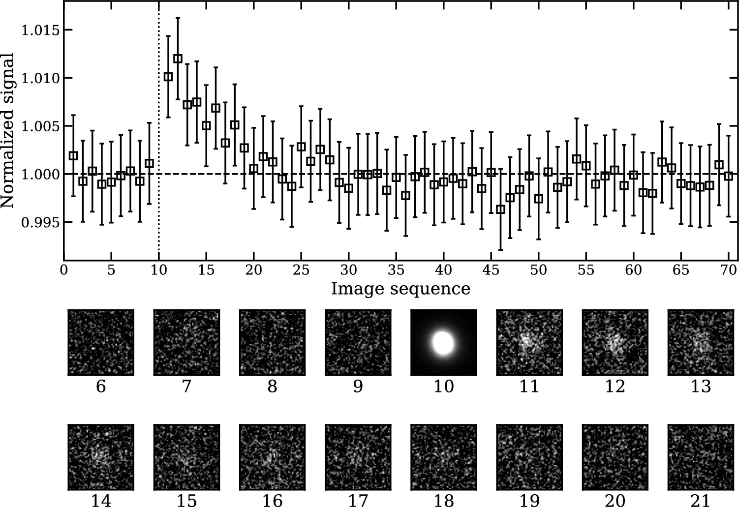
We investigate the residual signal remaining at the position of a bright source after exposure. A bright star is exposed (300 s) and a series of 30 s dark frames are obtained before (9 frames; Group A) and after (60 frames; Group B) the star's image. Figure 2 shows the signal variation with the image sequence within a 10 pixel diameter circular aperture (assuming 41 seeing) at the star's position in the pixel coordinates. Each data point is normalized with the mean value of Group A's signal, and the star's signal (Image sequence = 10) is not shown due to its high signal value (45.88). We find the residual signals in Group B shown in the image thumbnails in Figure 2. The signal of the first dark frame in Group B (Image sequence = 11) is 1% higher than the mean value of Group A's signal, resulting in a magnitude difference of 0.011 mag. The effect of the residual signal disappears within 3 times the standard deviation of Group A's signal after 8 readouts. Therefore, observers have to consider the residual signal for the photometry of the faint objects.

Figure 2. The signal variation with the image sequences for the residual signal. The error bars are photometric uncertainties of each data point. The vertical dotted line is the image sequence of the star, meaning that Group A and Group B are on the left and right sides of the vertical line, respectively. The horizontal dashed line is the mean value of Group A's signal. Thumbnails from the 6th to the 21st image are presented in a square box with a width of 50 pixels, which are Gaussian smoothed in a log scale.
Download figure:
Standard image High-resolution image2.2.3. Linearity
It is important to check if the input charges can be converted into the output electric signal with a simple linear relation. A series of dome-flat images taken with V-band are obtained by progressively increasing exposure time while the dome-flat lamps are turned on and the telescope is directed toward the dome-flat panel. Figure 3 shows a variation of mean counts of the dome-flat images from 0.1 to 240 s exposure. The pixels started to be saturated from 215 s exposure. The mean counts are well fitted with the linear relation up to ∼61,000 ADU within 2.5% and ∼57,000 ADU within 1% ( ). Even in the exposure time shorter than 1 s, the linearity can be found ≳100 ADU within 5%. During this process, any feature of the shutter pattern for the short-exposure images is not found.

Figure 3. The variation of the mean values of the dome-flat images is presented. The linear fit is overplotted in a red solid line from the exposure time of 0.2–210 s. The inset plot shows the linear relation for shorter exposures. The residual plot is also provided in the bottom panel.
Download figure:
Standard image High-resolution image2.2.4. Dark Current
We also investigate a variation of the dark current resulting from the thermal electron with the CCD cooling temperatures from −30°C to −1.1° C. At −20° C, the dark current is 0.01 e− pixel−1 s−1 as presented in Figure 4. The mean values from the bias-subtracted and combined dark frames (180 s exposure) are taken. The dark frame obtained at the lowest temperature (−30°C) is used as a reference to remove any other signals not dependent on the CCD temperature by subtracting those taken at the high temperature.

Figure 4. A variation of the dark current with the CCD temperature. The data points indicated by gray circles are obtained from the Kodak KAF-16803 Image Sensor Device Performance Specification document (https://www.onsemi.com/products/sensors/image-sensors/KAF-16801).
Download figure:
Standard image High-resolution image2.3. Filter System and Throughput
Currently, the filter wheel SBIG-FW7 attached to the CCD camera has a set of 5 broadband (Bessell UBVRI) and 3 narrow band filters (Hα, O iii, and S ii) manufactured by Chroma Technology, Co. with a size of 50 mm × 50 mm. The filter transmission curve altogether with the quantum efficiency (QE) of CCD and the telescope optics throughput is provided in Figure 5. For CCD, the QE peaks at 60% at 5500 Å. For optics throughput, the corrector lenses with the standard anti-reflection coatings and the first surface mirrors with the enhanced Aluminium reflective coatings are considered, showing the peak (82%) at 6000 Å.

Figure 5. Transmission curves of the broadband filter system at MAAO. The optics, CCD QE, and each filter are plotted with black dashed, solid, and dotted lines, respectively. The filter transmission is plotted before and after considering CCD QE and optics (colored solid lines). Note that the U-band throughput is not complete since the transmission of the optics and CCD QE is not provided in a wavelength range <3900 and <3490 Å.
Download figure:
Standard image High-resolution imageIn summary, the overall characteristics of the CCD camera on the MAAO 0.7 m telescope are presented in Table 1.
Table 1. Specifications of the Current CCD Camera (SBIG STX-16803)
| Properties | Values |
|---|---|
| Sensor chip | KAF-16803 (36.8 mm × 36.8 mm) |
| Pixel size | 9 μm × 9 μm |
| Pixel arrays | 4,096 × 4,096 |
| Readout time a | 9 s |
| QE peak | 60% |
| Pixel scale | 0 41 pixel−1
|
| Field of view | 279 × 279 |
| Gain | 1.30 ± 0.04 e− ADU−1 |
| Readout noise | 12.62 ± 0.25 e− |
| Linearity | 350−57,000 ADU (within 1%) |
| Full well a | 100,000 e− |
| Dark current | 0.01 e− pixel−1 s−1 at −20° C |
Note.
a The manufacturer's data are adopted.Download table as: ASCIITypeset image
3. System Integration and Robotic Observation
3.1. System Integration
Two personal computers (PCs) control the system in a 64-bit Windows operating system environment. One is the main control PC connected to the 0.7 m telescope system and the other is the automatic weather station (AWS) PC. Figure 6 summarizes the system configuration at MAAO.

Figure 6. A schematic of the system integration at MAAO. Solid boxes represent hardware, while dashed lines indicate computer files and software components, including scripts, data, and logs.
Download figure:
Standard image High-resolution image3.1.1. Telescope System
The 0.7 m telescope system is operated by a series of commercial software in the main control PC such as PlaneWave Interface 2 (PWI2), PWShutter, and MaxIm DL 6.26. We integrated all the instruments using Python scripts, as demonstrated below.
The mount, the derotator, the tertiary mirror, and the focuser are controlled by PWI2 over TCP/IP communication on a local network. PWI2 command is also supported by a Python script provided by PlaneWave Instruments. 10 The mirror cover control software, PWShutter, is connected in the same manner referring to the sample code provided in the PWShutter user manual.
For the CCD camera and the filter wheel control, MaxIm DL 6.26 11 is utilized using AStronomy Common Object Model (ASCOM) 12 standard driver, which provides universal interfaces for many astronomical devices. The ASCOM properties and methods in MaxIm DL can be translated into Python language via pywin32 13 module.
The dome is equipped with a Shelyak Dome Tracker in a serial connection for the ASCOM dome control. For the dome shutter and dome-flat lamps, they are independently controlled by an ethernet relay via TCP/IP communication using another IP address.
3.1.2. Weather Monitoring System
There are two components to the weather monitoring system: the Davis weather station for meteorological data and the all-sky camera for measuring cloud coverage.
The Davis weather station obtains temperature, humidity, wind speed/direction, and so on. This equipment is connected to the AWS PC via a Vantage Pro2 device on a serial port connection. We upload the weather data in real-time on the global network 14 via WeatherLink software. Then we retrieve this data via a Python script using WeatherLink APIv2 15 on the main control PC to give constraints on whether to open or close the dome.
Using the all-sky camera images, we detect the presence of clouds with a Python module of cloudynight 16 (Mommert 2020). The Python module uses a machine-learning model of lightGBM (Ke et al. 2017). The training and test data set will be addressed in the future work (Lim et al. in preparation). For in-person observations, observers can identify clouds in images visually.
The dome remains open when all of the following conditions are met: outside humidity <95%, outside temperature > −10°C, wind speed <15 m s−1, no cloud detection, and no detection of lightning within a radius <16 km around MAAO. 17
3.2. Robotic Observation
An one-day run of the robotic observation involves 7 sessions: StartUp, Observation, AutoFocus, Idle, CalFrame, ShutDown, and FileTransfer, and they are controlled by a scheduler. Figure 7 illustrates a sequence of these sessions.

Figure 7. A flowchart for the scheduler at MAAO and each session. Solid arrows show the path to the next step when the weather is safe, while dashed arrows represent the path under unsafe weather conditions.
Download figure:
Standard image High-resolution image(i) StartUp session can start when the solar altitude is below −18 deg and when the public event is finished (after 9 PM/10 PM in winter/summer). This session includes software initialization, azimuth synchronization of the dome and scope, dome opening, tertiary mirror position switching for CCD imaging, and CCD chip cooling. When the weather condition is poor, the scope enters Idle session.
(ii) Observation session performs observations based on scripts. The observation script, an ASCII file, must contain the following columns: object name (NAME), R.A. in J2000 (RA_J2000), decl. in J2000 (DEC_J2000), rise and set times above a specific altitude in local time (RISE(LT), SET(LT)), transit time (TRANSIT(LT)), filter (FILTER), single exposure time (EXPTIME), CCD binning (BINNING), the number of exposures to repeat (COUNTS), and observation starting time in local time (OBSTIME).
(iii) AutoFocus session uses the default auto-focusing function supported in PWI2. In the AutoFocus session, an optimal focus value can be determined by using a relationship between PSF sizes of a point source and focus values in a series of short exposure images. Users have the option to perform AutoFocus manually by generating an Observation session with "AutoFocus" in the NAME column. An initial auto-focusing procedure is performed every StartUp session.
(iv) CalFrame session takes calibration frames (bias, dark, and dome-flats) before ShutDown session. For dome-flats, after the dome closed, the scope points to the dome-flat panel (Azimuth = 267 deg, altitude = 51.5 deg), and the dome moves to the opposite position (Azimuth = 88.3 deg).
(v) Idle session moves the scope to the parking position, disables tracking, and closes the dome. The observation resumes when the weather conditions have remained safe for 30 minutes.
(vi) ShutDown session is set to automatically initiate when the solar elevation exceeds −18 deg.
(vii) FileTransfer session automatically sends observed data obtained during the nighttime using the file transfer protocol (FTP) to the server. The observation is summarized into an observation log and sent to the observer via email.
During the execution, the scheduler checks the solar altitude, local time, and weather data every 60 s to finish or halt the observation. An operation log is also generated after each command.
4. System Performances
We investigate PSF shape variations, atmospheric coefficients, zero-point magnitudes, and limiting magnitudes. Acquired raw data in this section is reduced with the standard image reduction and analysis facility routine using PyRAF package (Science Software Branch at STScI 2012) of bias, dark, and flat-field correction. Although it is known that observations at IR wavelengths can be affected by fringe patterns (e.g., Figure 13 in Im et al. 2010), we find no significant fringe pattern even in I-band images, and therefore, no fringe pattern correction is applied. Astrometric solution is entered using Astrometry.net (Lang et al. 2010). The data in this work are reduced in this manner.
4.1. Optical Performance
To explore the optical performance and tracking accuracy, we obtain the images with extending exposure times from 5 to 600 s, including 10, 30, 60, 120, 180, and 300 s. The left panel in Figure 8 shows the total FOV divided into 16 image sections a 60 s exposure of an open cluster NGC 0884. The PSF model in each section is built using PSFEx (Bertin 2013) from the detected stars with a high S/N ratio at least 20 but not saturated by setting the PSFEx parameters of SAMPLE_MINSN = 20 and SATUR_LEVEL = 50000, respectively. The right panel shows the PSF models produced in each image section with the ellipticity values (ELLIPTICITY from SExtractor, Bertin & Arnouts 1996). Though the PSF shape on the left-bottom side is slightly elongated (0.1 at maximum), we find uniform PSF shapes over the FOV.

Figure 8. Left: The total FOV of the CCD camera for the R-band image divided into 16 sections. The mean full-width half maximum (FWHM) value in the total field is 29 for the 60 s exposure time. Right: PSF images built from stars in each division. The number presents the ellipticity of the PSF.
Download figure:
Standard image High-resolution image4.2. Photometric Calibration
Photometric calibration is required because the photometric system depends on the characteristics of optics, imaging devices, and observing conditions. To measure the photometric parameters using data obtained at MAAO, we observed several standard star fields (SA 23 and SA 35) presented in Landolt (2013). The observations were performed in the clear sky, and the observation information is summarized in Table 2. After data reduction, we measure the magnitudes of the standard stars using the SExtractor with the 14'' diameter circular aperture to match with the same size aperture in Landolt (2013). We obtained the photometric parameters using the following equations:


Table 2. Observation Logs of Standard Stars (SA 23 and SA 35)
| Epoch | Filter | Date-Obs (UT) | MJD | Airmass | FWHM ('') | Exposures |
|---|---|---|---|---|---|---|
| 1 | B | 2023-02-20 10:38:37 | 59995.443 | 1.06 | 3.18 | 60 s × 3 |
| V | 2023-02-20 10:45:21 | 59995.448 | 1.07 | 3.03 | ||
| 2 | B | 2023-02-20 12:17:41 | 59995.512 | 1.24 | 3.69 | 60 s × 3 |
| V | 2023-02-20 12:21:26 | 59995.515 | 1.25 | 3.57 | ||
| 3 | B | 2023-02-20 13:38:13 | 59995.568 | 1.57 | 2.86 | 60 s × 3 |
| V | 2023-02-20 13:42:22 | 59995.571 | 1.59 | 2.98 | ||
| 4 | B | 2023-02-20 14:17:47 | 59995.596 | 1.84 | 4.14 | 60 s × 3 |
| V | 2023-02-20 14:21:51 | 59995.599 | 1.87 | 3.90 | ||
| 5 | B | 2023-02-20 14:39:39 | 59995.611 | 2.03 | 3.56 | 60 s × 3 |
| V | 2023-02-20 14:44:40 | 59995.614 | 2.09 | 3.85 | ||
| 1 | B | 2023-03-28 13:13:48 | 60031.551 | 2.19 | 3.48 | 60 s × 5 |
| V | 2023-03-28 13:19:54 | 60031.555 | 2.12 | 2.74 | ||
| R | 2023-03-28 13:26:01 | 60031.560 | 2.05 | 3.71 | ||
| I | 2023-03-28 13:32:08 | 60031.564 | 1.99 | 3.09 | ||
| 2 | B | 2023-03-28 13:57:20 | 60031.581 | 1.77 | 3.64 | 60 s × 5 |
| V | 2023-03-28 14:03:28 | 60031.586 | 1.73 | 3.66 | ||
| R | 2023-03-28 14:09:35 | 60031.590 | 1.68 | 3.56 | ||
| I | 2023-03-28 14:15:41 | 60031.594 | 1.64 | 3.51 | ||
| 3 | B | 2023-03-28 14:23:32 | 60031.600 | 1.59 | 4.31 | 60 s × 5 |
| V | 2023-03-28 14:29:39 | 60031.604 | 1.56 | 3.72 | ||
| R | 2023-03-28 14:35:46 | 60031.608 | 1.53 | 3.34 | ||
| I | 2023-03-28 14:41:52 | 60031.612 | 1.49 | 2.95 | ||
| 4 | B | 2023-03-28 14:55:39 | 60031.622 | 1.43 | 3.51 | 60 s × 5 |
| V | 2023-03-28 15:01:46 | 60031.626 | 1.40 | 3.56 | ||
| R | 2023-03-28 15:07:53 | 60031.630 | 1.38 | 3.50 | ||
| I | 2023-03-28 15:13:60 | 60031.635 | 1.35 | 3.09 | ||
| 5 | B | 2023-03-28 16:01:28 | 60031.668 | 1.21 | 3.81 | 60 s × 5 |
| V | 2023-03-28 16:07:34 | 60031.672 | 1.19 | 3.29 | ||
| R | 2023-03-28 16:13:41 | 60031.676 | 1.18 | 2.75 | ||
| I | 2023-03-28 16:19:48 | 60031.680 | 1.16 | 2.84 | ||
| 1 | B | 2024-03-20 13:40:44 | 60389.570 | 2.22 | 4.42 | 120 s × 5 |
| V | 2024-03-20 13:51:50 | 60389.578 | 2.09 | 4.15 | ||
| R | 2024-03-20 14:02:56 | 60389.582 | 2.02 | 4.07 | ||
| I | 2024-03-20 14:14:02 | 60389.590 | 1.91 | 4.04 | ||
| 2 | B | 2024-03-20 14:29:45 | 60389.604 | 1.75 | 4.17 | 120 s × 5 |
| V | 2024-03-20 14:40:51 | 60389.612 | 1.67 | 3.52 | ||
| R | 2024-03-20 14:51:56 | 60389.616 | 1.63 | 3.36 | ||
| I | 2024-03-20 15:03:02 | 60389.624 | 1.56 | 3.53 | ||
| 3 | B | 2024-03-20 15:23:52 | 60389.642 | 1.43 | 3.96 | 120 s × 5 |
| V | 2024-03-20 15:34:58 | 60389.649 | 1.38 | 3.89 | ||
| R | 2024-03-20 15:46:04 | 60389.654 | 1.36 | 3.64 | ||
| I | 2024-03-20 15:57:10 | 60389.662 | 1.32 | 2.41 | ||
| 4 | B | 2024-03-20 16:18:30 | 60389.680 | 1.24 | 3.83 | 120 s × 5 |
| V | 2024-03-20 16:29:36 | 60389.687 | 1.21 | 3.45 | ||
| R | 2024-03-20 16:40:42 | 60389.692 | 1.19 | 2.90 | ||
| I | 2024-03-20 16:51:48 | 60389.700 | 1.17 | 2.63 | ||
Download table as: ASCIITypeset image
In these equations, the observed magnitudes are denoted as b, v, r, and i and the standard magnitudes are B, V, R, and I provided from Landolt (2013). Additionally, zB
, zV
, zR
, and zI
correspond to the zero-points for the magnitudes producing a signal of 1 e- s−1 in each band.  ,
,  ,
,  , and
, and  are the first-order atmospheric extinction coefficients and
  ,
,  ,
,  , and
, and  are the second-order atmospheric extinction coefficients. Since the second-order extinction coefficients are small, they can be negligible. The color term coefficients are CB
, CV
, CR
, and CI
, and X represents the airmass. Table 3 presents the resultant of the calibration.
are the second-order atmospheric extinction coefficients. Since the second-order extinction coefficients are small, they can be negligible. The color term coefficients are CB
, CV
, CR
, and CI
, and X represents the airmass. Table 3 presents the resultant of the calibration.
Table 3. The Resultants of Standard Calibration
| Filter |

| C | k'' | z | Nstar | σrms |
|---|---|---|---|---|---|---|
| B | 0.477 ± 0.032 | 0.011 ± 0.070 | −0.070 ± 0.047 | −21.632 ± 0.049 | 11 | 0.028 |
| V | 0.328 ± 0.013 | 0.102 ± 0.027 | −0.016 ± 0.017 | −21.912 ± 0.021 | 14 | 0.021 |
| B | 1.375 ± 0.086 | −0.182 ± 0.237 | −0.038 ± 0.138 | −21.911 ± 0.148 | 7 | 0.039 |
| V | 1.068 ± 0.041 | 0.197 ± 0.099 | −0.090 ± 0.057 | −22.181 ± 0.071 | 7 | 0.016 |
| R | 0.752 ± 0.028 | 0.012 ± 0.121 | 0.084 ± 0.069 | −21.861 ± 0.049 | 7 | 0.010 |
| I | 0.642 ± 0.088 | 0.192 ± 0.118 | −0.100 ± 0.067 | −21.081 ± 0.088 | 7 | 0.019 |
| B | 0.560 ± 0.036 | −0.163 ± 0.086 | 0.031 ± 0.053 | −21.777 ± 0.059 | 7 | 0.019 |
| V | 0.311 ± 0.020 | −0.007 ± 0.045 | 0.072 ± 0.028 | −21.960 ± 0.032 | 7 | 0.011 |
| R | 0.221 ± 0.027 | 0.024 ± 0.107 | 0.110 ± 0.066 | −21.865 ± 0.044 | 7 | 0.012 |
| I | 0.120 ± 0.022 | −0.014 ± 0.048 | 0.036 ± 0.029 | −20.912 ± 0.037 | 7 | 0.009 |
Note. Nstar is the Number of Stars used in the Calibration Process.
Download table as: ASCIITypeset image
Figure 9 shows the residuals of the measured magnitudes in each observing date. The extinction coefficients measured on 2023 February 20th and 2024 March 20th are comparable to those measured in other Korean observatories (See Table 4). Considering the analysis in Kim et al. (2008), the heavy extinction observed on 2023 February 28th might be related to a considerable amount of fine dust in spring season or the possibility of thin cirrus clouds.

Figure 9. The residual plot of the transformation into the standard system.
Download figure:
Standard image High-resolution imageTable 4. The First-order Atmospheric Extinction Coefficients in Multiple Filters for Korean Observatories in Units of mag per Airmass
| Site | No Filter | B | V | R | I | References |
|---|---|---|---|---|---|---|
| CBNUO a | 0.34–0.45 | Kim et al. (2008) | ||||
| BOAO b , c | ∼0.30 | ∼0.20 | ∼0.10 | <0.10 | Kim et al. (1997) | |
| SNU d | 0.36–0.90 | 0.73 | Lee et al. (2009) | |||
| GAO e | 0.20 | 0.13 | Lee et al. (2007) | |||
| DOAO f | 0.88 | 0.64 | Kwon (2014) g | |||
| MAAO | 0.48–1.38 | 0.31–1.07 | 0.22–0.75 | 0.12–0.64 | This work |
Notes.
a Chungbuk National University Observatory. b Bohyunsan Optical Astronomy Observatory. c We adopted values at the nearest wavelength from Table 3 in Kim et al. (1997). d Department of Earth Science Education, Seoul National University. e Gimhae Astronomical Observatory. f Deokheung Optical Astronomy Observatory. g Research Report 2014 of the National Youth Space Center (NYSC), https://nysc.kywa.or.kr/organ/data.jsp.Download table as: ASCIITypeset image
4.3. Limiting Magnitudes
We measure limiting magnitudes of images in BVRI-band. A spiral galaxy NGC 3147 was observed in 10 minutes exposure under a clear dark night on 2023 February 20th as shown in the left panel in Figure 10. We perform the photometry using the SExtractor with a 2 × FWHM aperture diameter. The FWHM values exhibit variation ranging from 28 to 38 with the filter and the focus. The photometric catalog from the Data Release 1 of Pan-STARRS
18
(PS1; Tonry et al. 2012) is used as a reference catalog to calculate the zero-point magnitudes. We convert PS1 gri magnitudes to BVRI magnitudes (Refer Section 2.1 in Lim et al. 2023). As a result, the 5σ limiting magnitude in R-band for the 10 minutes exposure can be achieved as ∼20 mag, which is comparable to that of other telescopes measured in Korea (Refer Table 1 in Im et al. 2021). The other measured limiting magnitudes are summarized in Table 5.

Figure 10. Sample images obtained from the 0.7 m telescope. Left: BVR-bands color image for the ambiance of NGC 3147 used for measuring the limiting magnitudes on 2023 February 20th in Section 4.3. Right: VRI-bands color image of M101 on 2023 May 20th. SN 2023ixf is marked in a yellow reticle.
Download figure:
Standard image High-resolution image
Table 5. The Limiting Magnitudes of Images Obtained from the MAAO 0.7 m Telescope in UBVRI-bands before and after Cleaning the Mirror
| Filter | Date-Obs (UT) | Zero Point (AB) | FWHM ('') | Exposures | 5σ Limit (AB) |
|---|---|---|---|---|---|
| U | 2023-03-29 13:01:26 | 16.63 ± 0.17 | 3.10 ± 0.04 | 600 s × 5 + 300 s × 20 | 16.76 |
| B | 2023-02-20 14:55:26 | 20.87 ± 0.07 | 3.31 ± 0.06 | 120 s × 5 | 19.48 |
| V | 2023-02-20 15:07:11 | 21.28 ± 0.03 | 3.84 ± 0.06 | 19.36 | |
| R | 2023-02-20 15:18:53 | 21.44 ± 0.02 | 3.66 ± 0.07 | 19.64 | |
| I | 2023-02-20 14:31:11 | 20.89 ± 0.02 | 2.85 ± 0.06 | 19.59 | |
| B | 2023-06-16 13:39:38 | 21.25 ± 0.05 | 2.59 ± 0.04 | 60 s × 5 | 18.08 |
| V | 2023-06-16 13:45:41 | 21.66 ± 0.04 | 2.52 ± 0.04 | 18.34 | |
| R | 2023-06-16 13:52:01 | 21.87 ± 0.05 | 2.58 ± 0.08 | 18.53 | |
| I | 2023-06-16 13:58:04 | 21.16 ± 0.03 | 2.54 ± 0.05 | 18.29 | |
Download table as: ASCIITypeset image
The U-band limiting magnitude is 16.8 AB mag. Due to the low sensitivity of the U-band, all the U-band images of SA 32 field obtained on 2023 March 29th with the total integrate time of 150 minutes are stacked. The zero-point magnitude is measured using the magnitudes of standard stars from Landolt (2013) and is converted into the AB system using Blanton & Roweis (2007).
After cleaning the mirror on 2023 May 30th, we additionally measured the limiting magnitudes of 5 minutes exposure images of M101 field on 2023 June 16th. We calibrated the observed magnitudes with the same manner using the stars in the data release 9 (DR9) of the AAVSO photometric all-sky survey (Henden et al. 2016) as comparison stars. The zero-points showed an improvement of ∼0.4 mag.
5. Current Scientific Programs
We describe current research topics mainly focusing on time-series observational studies, including supernovae (SNe) and transiting exoplanets.
(i) Supernovae: The MAAO 0.7 m telescope participates in a high-cadence monitoring program of nearby galaxies to obtain light curves of supernovae (SNe) in their infant phase, as part of a telescope network (Im et al. 2019, 2021). Monitoring the rising part of their light curves allows us to constrain SN progenitor models (Im et al. 2015; Lim et al. 2023). One recent detection is SN 2023ixf (Type II), the nearest supernova in the last 10 yr. As soon as we received the transient alert, we captured the very early light of SN 2023ixf within a day of its discovery on 2023 May 19th (Itagaki 2023) (see the right panel of Figure 10 for a sample VRI-band color image of M101, the host galaxy). This early data will contribute to our understanding of the fate of massive stars (Kim et al. in preparation).
(ii) Transiting Exoplanets: Space-based telescopes searching for transiting exoplanets such as Kepler (Borucki et al. 2010) and TESS (Ricker et al. 2015) have monitored a large number of stars with high-cadence and high photometric precision for many years, discovering more than thousands of the exoplanets and objects of interests showing planetary features. The light curves and stellar and planetary parameters of these objects are published in databases (e.g., NASA Exoplanet Archive; Akeson et al. 2013). However, due to the limitation of their lifetime and originally designed mission, the targets have been monitored with a limited time duration and filters. So their photometric follow-up observation with small telescopes can allow us to confirm them as exoplanets and characterize their physical properties (mass, radius, density, etc.) and orbital ephemerides. We are now performing a pilot observation of a confirmed transiting exoplanet to examine the capabilities of MAAO.
6. Future Work
Future work involves a long-term monitoring of observing conditions and system stabilization. The study of the seasonal change of the astronomical seeing (Lim et al. in preparation), atmospheric extinction coefficients, and the influence of light pollution on the sky brightness at MAAO (Park et al. in preparation) are ongoing. These studies would provide observers with insights into establishing observation strategies, and reference materials for MAAO staff to maintain the instrument and educate the public in consideration of local weather conditions.
7. Summary and Conclusion
We present the performance of the 0.7 m robotic telescope system at MAAO and its standard photometric system, and current science programs. The 0.7 m telescope is newly installed at MAAO, a public observatory in Miryang, Korea. We have established a robotic observing system to utilize this system for scientific observations following public events. The gain, readout noise, residual signal, dark current of the detector, and the total throughput are also evaluated. We find that the PSF shape is spatially uniform across the overall FOV with an ellipticity of <0.1 for a 1 minutes exposure time. Subsequently, photometric calibration is performed using standard stars in the BVRI-band. The atmospheric extinction coefficients are moderate compared to those of other observatories in Korea, but we find severe extinction which needs to be confirmed with future data. The 0.7 m telescope can achieve image depths down to BVRI ∼ 19.4–19.6 AB mag at 5σ with a 10 minutes integrated time under clear dark sky conditions and a seeing condition of ∼29–38, comparable to those of other Korean observatories used for research. Due to the low system sensitivity in ultraviolet, the U-band depth is shallow (U ∼ 16.8 AB mag) even with a 150 minutes exposure time. While the MAAO system serves as a public facility, our automation efforts make it available for astronomical research, especially for time-domain astronomy such as, supernova monitoring and transiting exoplanets. In the future, we plan to stabilize the automated observation.
Acknowledgments
This work acknowledges support from the Basic Science Research Program through the National Research Foundation of Korea (NRF) funded by MSIT (No. 2022R1A6A3A01085930). D.K. acknowledges support by the NRF of Korea (NRF) grant (Nos. 2021R1C1C1013580 and 2022R1A4A3031306) funded by MSIT. M.I. and H.C. acknowledge the support from the National Research Foundation of Korea (NRF) grants, No. 2020R1A2C3011091, and No. 2021M3F7A1084525, funded by the Korea government (MSIT). We sincerely thank the MAAO staff and Metaspace, Inc. for the kind assistance and maintenance of the facilities. The authors also thank Bill Dean of PlaneWave Instruments for providing us with the response curve of the telescope.
Facility: MAAO:0.7m - .
Software: Astrometry.net (Lang et al. 2010), cloudynight (Mommert 2020), SExtractor (Bertin & Arnouts 1996), PSFEx (Bertin 2013), PyRAF (Science Software Branch at STScI 2012), WeatherLink APIv2 (https://weatherlink.github.io/v2-api/), pywin32 (https://github.com/mhammond/pywin32).
Footnotes
- 10
- 11
- 12
- 13
- 14
- 15
- 16
- 17
We adapted the radius in the Lick observatory (https://mthamilton.ucolick.org/techdocs/telescopes/Nickel/limits_weather/) which is related to the standard lightning alert radius (DiGangi et al. 2022).
- 18