KPS-1b: The First Transiting Exoplanet Discovered Using an Amateur Astronomer's Wide-field CCD Data

Artem Burdanov; Paul Benni; Eugene Sokov; Vadim Krushinsky; Alexander Popov; Laetitia Delrez; Michael Gillon; Guillaume Hébrard; Magali Deleuil; Paul A. Wilson; Olivier Demangeon; Özgür Baştürk; Erika Pakštiene; Iraida Sokova; Sergei A. Rusov; Vladimir V. Dyachenko; Denis A. Rastegaev; Anatoliy Beskakotov; Alessandro Marchini; Marc Bretton; Stan Shadick; Kirill Ivanov

doi:10.1088/1538-3873/aabde2

1. Introduction

A major fraction of all exoplanets confirmed to date transit their host stars (Schneider et al. 2011; Akeson et al. 2013; Han et al. 2014). The eclipsing configuration of these planets enables us to measure their radii and masses by combining prior pieces of knowledge on their host star properties with photometric and radial velocity measurements, and thus to constrain their bulk compositions (Winn 2010). With sufficient signal to noise ratios (S/N), it is also possible to explore their atmospheric properties (Winn 2010; Burrows 2014; Madhusudhan et al. 2016).

Despite their rarity in the Milky Way (∼1% occurrence rate, e.g., Wright et al. 2012), hot Jupiters (i.e., planets with minimum mass M sin i > 0.5 M_Jup and orbital period P ≲ 10 days) are particularly favorable targets for non-space surveys. It is due to their short orbital periods that maximize their transit probabilities, and to their large sizes (up to 2 R_Jup) that maximize their transit depths. These short period gas giants orbit in strong gravitational and magnetic fields (Chang et al. 2010; Correia & Laskar 2010) and undergo irradiation larger than any planet in the Solar System (Fortney et al. 2007). Thorough characterization of hot Jupiters gives us an opportunity to research the response of these planets to severe environments, and to find out their planetary structures and chemical compositions. Moreover, their orbital obliquity can be measured during their transits (Hébrard et al. 2008, 2011; Moutou et al. 2011; Sanchis-Ojeda & Winn 2011; Sanchis-Ojeda et al. 2011), bringing a key constraint on their dynamical history (Triaud et al. 2010).

Approximately 300 transiting hot Jupiters are known to date. Wide-field photometric surveys operating from the ground, such as WASP (Pollacco et al. 2006), HAT (Bakos et al. 2004; Bakos et al. 2013), KELT (Siverd et al. 2012), Qatar (Alsubai et al. 2013), XO (McCullough et al. 2005; Crouzet 2017) and TrES (Alonso et al. 2004) discovered most of them. Space missions, namely CoRoT (Auvergne et al. 2009), Kepler (Borucki et al. 2010) and K2 (Howell et al. 2014) also contributed to the number of known hot Jupiters. However, the combination of these surveys has left a significant fraction of the sky—the Galactic plane (see Figure 1)—relatively unexplored. Indeed, all these wide-field surveys, including future space missions like PLATO (Rauer et al. 2014) and TESS (Ricker et al. 2015), have a poor spatial resolution in common. It translates into a large level of blending for the crowded fields of the Galactic plane, resulting into a poorer detection potential (due to signal dilution) combined with a drastically increased level of false-alarm probability (due to blended eclipsing binaries). For these reasons, most of the cited surveys try to avoid fields of low Galactic latitudes. Hence, many more hot Jupiters still remain undiscovered there.

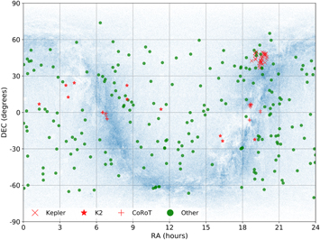
**Figure 1.** Transiting hot Jupiters known to date on a projection of the celestial sphere. The exoplanet sample is from the NASA Exoplanet Archive (Akeson et al. 2013) and stars' positions are from the Tycho-2 catalog (Høg et al. 2000).
Download figure:
Standard image High-resolution image

This work is based on the hypothesis that amateur astronomy could play a significant role in their discovery. The synergy between amateur and professional astronomers in the exoplanetary research field has proven to be fruitful (Croll 2012). Some examples of that are Zooniverse-based¹⁸ projects Planet Hunters (Fischer et al. 2012) and Exoplanet Explorers.¹⁹ Amateurs also participate in the ground-based exoplanet follow-up—for example, KELT-FUN observations for KELT exoplanet candidates (McLeod et al. 2017), observations of KOI-1257 b Kepler exoplanet candidate (Santerne et al. 2014), and take an active part in search for Transit Timing Variations (Baluev et al. 2015). However, aforementioned projects are focused on searching for planets in already existing data sets, observing exoplanet candidates and already known planet-bearing stars discovered by professional astronomers. Now amateurs can also contribute to the search for transiting exoplanets by directly gathering wide-field CCD data. This approach is used by the PANOPTES (Guyon et al. 2014) project and the project described in this paper.

In 2012–2016 we carried out the Kourovka Planet Search (KPS, Popov et al. 2015; Burdanov et al. 2016)—a prototype survey with the primary objective of searching for new transiting exoplanets in the fields of low Galactic latitudes. We used the MASTER-II-Ural robotic telescope (Gorbovskoy et al. 2013) operated at the Kourovka astronomical observatory of the Ural Federal University in the Middle Urals (Russia). At first our observations of target fields TF1 and TF2 in the Galactic plane were performed solely with the MASTER-II-Ural telescope. But since 2014 the Rowe-Ackermann Schmidt Astrograph, operated at the private Acton Sky Portal Observatory (MA, USA), joined the project by observing an additional target field TF3 (located not in the Galactic plane, but in the Ursa Major constellation). Exoplanet candidates that were discovered in the fields TF1 and TF2 turned out to be astrophysical false positives. Here we announce the discovery of the transiting hot Jupiter KPS-1b, which was found after analyzing the TF3 wide-field CCD data gathered at the private Acton Sky Portal Observatory.

The rest of this paper is structured as follows: information about initial detection observations and subsequent follow-up observations are given in Section 2; data analysis and derived parameters of planetary system are presented in Section 3; and in Section 4, we briefly discuss the discovered planetary system, outline evolution of the KPS project and future prospects.

2. Observations

2.1. KPS Transit Detection Photometry

As a part of the KPS prototype survey, we observed target field #3 (TF3), which is located in the Ursa Major constellation and contains the smallest number of stars of all the fields observed within the survey. This field is not in the plane of the Milky Way (poorly observable in the northern hemisphere at the time), but was nonetheless observed as part of the test observations with the Rowe-Ackermann Schmidt Astrograph (RASA) telescope for 21 nights in the period from 2015 January to April in the R_c filter and with 50 s exposures. The RASA telescope (Celestron Inc., Torrance, CA, USA) has a Schmidt-like optical design with a diameter of 279 mm and focal a length of 620 mm coupled with a Celestron CGEM mount. The telescope is based at the Acton Sky Portal private observatory in Acton, MA (USA). Software control of the telescope targeting and imaging was done by TheSkyX (Software Bisque, Golden, CO, USA). We used a SBIG ST-8300M camera (Santa Barbara Imaging Group, Santa Barbara, CA, USA) mounted on a custom adapter with a R_c filter. One 1.67 × 1.26 deg² field was imaged with a pixel resolution of 1 farcs 79 pixel⁻¹. Typical full width at half maximum (FWHM) of the stellar point-spread function values in the images were 2''–3''.

We used Box-fitting Least Squares method (BLS, Kovács et al. 2002) to search for periodic transit-like signals in our time-series and found a significant peak in the periodogram of the star KPS-1 (KPS-TF3-663 = 2MASS 11004017+6457504 = GSC 4148-0138 = UCAC4775-030421, Figure 2 and Table 1) located in the TF3 field. We detected five ∼0.01 mag transit-like events, two of them were full, which allowed us etimate the period as ∼1.7 days. The phase folded light curve with this period is shown in Figure 3. The details of data reduction, transiting signals search and research of exoplanet candidates can be found in Burdanov et al. (2016).

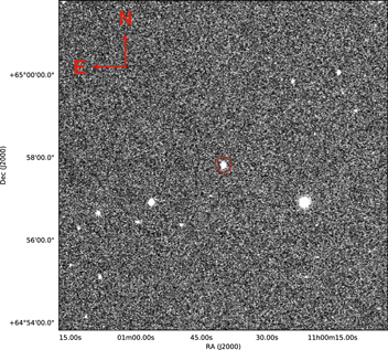
**Figure 2.** Finding chart including KPS-1 host star as obtained with the MTM-500 telescope in V band.
Download figure:
Standard image High-resolution image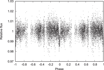

**Figure 3.** Phase folded RASA telescope photometry for KPS-1b.
Download figure:
Standard image High-resolution image

Table 1. General Information about KPS-1

Identifiers	KPS-1
	KPS-TF3-663^a
	2MASS11004017+6457504
	UCAC4775-030421
R.A. (J2000)	11^h 00^m 40176
Decl. (J2000)	+64^d 57^m 5047
Bmag^b	13.949
Vmag^b	13.033
Jmag^c	11.410

Notes.

^aExoplanet candidate ID from Burdanov et al. (2016). ^bData from the APASS catalog (Henden et al. 2016). ^cData from the 2MASS catalog (Cutri et al. 2003).

Download table as: ASCII Typeset image

2.2. Photometric Follow-up Observations

We conducted a set of photometric follow-up runs to validate transit-like events visible in our wide field data, check for presence of the secondary minimum to reject possible eclipsing binary scenario and then to analyze the shape of the transit signal. For this purpose we used a network of telescopes established within the framework of the KPS survey (for a full list of telescopes see Burdanov et al. 2016).

To determine the system's parameters, we used only high-precision photometric observations. These observations were conducted with the 1 m T100 telescope located at the TÜBİTAK National Observatory (Turkey) and the 1.65 m telescope located at the Molėtai Astronomical Observatory (Lithuania).

T100 is the 1 m Ritchey–Chrétien telescope at the TÜBİTAK National Observatory of Turkey located at an altitude of 2500 m above the sea level. The telescope is equipped with a high quality Spectral Instruments 1100 CCD detector, which has 4096 × 4037 matrix of 15 μm sized pixels. It was cooled down to −95° C with a Cryo-cooler. The pixel scale of the telescope is 0 farcs 31 pixel⁻¹, that translates into 21.5 × 21.5 arcmin² field of view (FOV). We used 2 × 2 binning in order to reduce the read-out time to 15 s, which also resulted in a better timing resolution. The star image was slightly defocused to limit the systematic noise originating from pixel to pixel sensitivity variations. To compensate the defocussing, the exposure time was increased to 26, 13, and 14 s in the ASAHI²⁰ SDSS $g^{\prime} ,r^{\prime} ,\mathrm{and}\,i^{\prime}$ filters respectively in the transit observations of KPS-1b on 2016 April 17. A Johnson R_c filter was used to observe a transit of KPS-1b on 2016 March 31 with 90 s exposure time. T100 has a very precise tracking system, improved even further by its auto-guiding system based on the short-exposure images acquired by an SBIG ST-402M camera. Thanks to this guiding system, the target was maintained within a few pixels during both observing runs. Data reduction consisted of standard calibration steps (bias, dark and flat-field corrections) and subsequent aperture photometry using IRAF/DAOPHOT (Tody 1986). Comparison stars and aperture size were selected manually to ensure the best photometric quality in terms of the flux standard deviation of the check star 2MASS J10595770+6455208, i.e., non-variable star similar in terms of magnitude and color to the target star.

Observations of KPS-1b transit on 2016 April 29 were conducted at the Molėtai Astronomical Observatory (MAO, Lithuania) with the 1.65 m Ritchey–Chrétien telescope. The telescope is equipped with the Apogee Alta U47-MB thermoelectrically cooled CCD camera, which has 1024 × 1024 matrix of 13 μm sized pixels. The pixel scale of the telescope is 0 farcs 51 pixel⁻¹, what gives 8.7 × 8.7 arcmin² FOV. Observations were conducted using a Johnson B filter with 60 s exposure time. The observed images were processed with the Muniwin program v. 2.1.19 of the software package C-Munipack (Hroch 2014). Reduction also consisted of standard calibration steps and subsequent aperture photometry.

Obtained light curves show 1.3%-depth achromatic transits. The light curves with imposed models and used baseline models (see Section 3.2 for details) are presented in Figure 4.

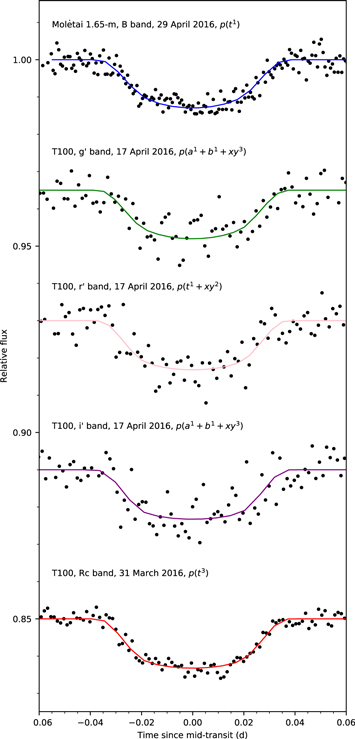
**Figure 4.** Transits of KPS-1b in different bands as obtained with T100 telescope of TÜBİTAK National Observatory of Turkey and 1.65 m Ritchey–Chrétien telescope of the Molėtai Astronomical Observatory (MAO, Lithuania). The observations are period-folded, multiplied by the baseline polynomials, and are shown in black. For each transit, the solid line represents the best-fit model. Along with the information about filter used, the baseline function is given (see Section 3.2 for details): p(x^N) stands for a N-order polynomial function of airmass (x = a), positions of the stars on CCD (x = xy), time (x = t) and sky background (x = b).
Download figure:
Standard image High-resolution image

As part of the KPS exoplanet candidates vetting, we perform photometric observations during the times of possible secondary minimums. Visual inspections of such light curves help to reveal obvious eclipsing binary nature of some of the candidates (for example, KPS-TF1-3154 and KPS-TF2-11789 from Burdanov et al. 2016). We observed KPS-1 at the expected time of secondary minimum on 2015 May 15. We used the 279 mm Celestron C11 telescope at the Acton Sky Portal. The telescope is equipped with the SBIG ST8-XME (Diffraction Limited/SBIG, Ottawa, Canada) thermoelectrically cooled CCD camera, which has 1530 × 1020 matrix of 9 μm sized pixels. FOV is 24.2 × 16.2 arcmin² with the pixel scale of 0 farcs 95 pixel⁻¹. Observations were conducted using an Astrodon Blue-blocking Exo-Planet filter²¹ which has a transmittance over 90% from 500 nm to beyond 1000 nm with 40 s exposure times. The observed images were processed in the similar way as the images from T100 and 1.65 m telescope, but with the AIP4WIN2 program (Willmann-Bell, Inc. Richmond, VA USA). These observations produced no detection (see Figure 5) and allowed us to rule out any eclipsing binary scenario with secondary eclipses deeper than 1% (3-sigma upper limit), thus strengthening the planetary hypothesis.

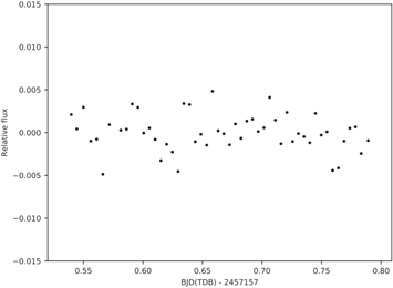
**Figure 5.** Light curve of KPS-1 during the time of a possible secondary minimum (mid-eclipse time BJD_TDB = 2457157.7284 ± 0.0005). Data was obtained with the 279 mm Celestron C11 telescope at the Acton Sky Portal (Acton, MA USA) in blue-blicking exoplanet filter and binned per 7 minutes intervals.
Download figure:
Standard image High-resolution image

2.3. Speckle-interferometric Observations

On 2015 June 7, we conducted speckle-interferometric observations of KPS-1 host-star with the 6 m telescope of the SAO RAS. We used a speckle interferometer based on EMCCD (Maksimov et al. 2009) with a new Andor iXon Ultra DU-897-CS0 detector. Observations were carried out in a field of 4.5 × 4.5 arcsec² in 800 nm filter with a bandwidth of 100 nm. We obtained two series of speckle images with exposure times of 20 and 100 milliseconds. During the analysis of power spectra we did not find any components at an angular distance up to 0 farcs 04 with a brightness difference of up to 3 mag and at a distance of up to 0 farcs 06 with a brightness difference of up to 4 mag (see Figure 6).

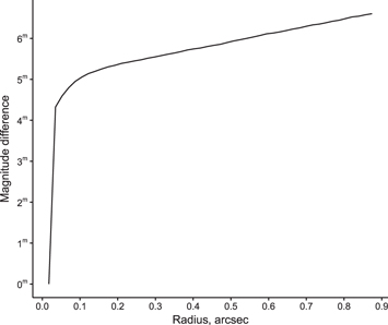
**Figure 6.** Autocorrelation function derived from the power spectrum by Fourier transform of KPS-1 star are calculated, translated to the 3σ detection limit Δm₃ and plotted as a function of radius.
Download figure:
Standard image High-resolution image

2.4. Spectroscopic Observations

We carried out spectroscopic follow-up observations of KPS-1 with the SOPHIE high-resolution spectrograph mounted on the 1.93 m telescope at the Haute-Provence Observatory in south-eastern France (Bouchy et al. 2009). This instrument provides high-precision radial velocity measurements, which allowed us to determine the planetary nature of the event and then to characterize the secured planet by measuring its mass and constraining its eccentricity.

Observations of KPS-1 with SOPHIE were conducted in the High-Efficiency mode (resolving power R = 40,000). Ten spectra were secured between 2016 March and July, with exposure times ranging from 1150 to 2340 s depending on the weather conditions. The SOPHIE automatic pipeline was used to extract the spectra. S/N per pixel at 550 nm were between 13 and 25 depending on the exposures, with typical values around 23. The weighted cross-correlation function (CCF) with a G2-type numerical mask was used to measure the radial velocities (Baranne et al. 1996; Pepe et al. 2002). Due to poor S/Ns, we removed 12 bluer of the 38 spectral orders from the CCF; this improved the accuracy of the radial-velocity measurement but did not significantly change the result by comparison to CCFs made on the whole SOPHIE spectral range.

We computed the error bars on radial velocities and the CCF bisectors following Boisse et al. (2010). Moonlight affected six spectra, but this contamination was corrected using the second fiber aperture pointing the sky during the observations (Hébrard et al. 2008; Pollacco et al. 2008). It allowed us to introduce large radial velocity corrections from 100 up to 650 m s⁻¹.

The radial velocity measurements and the CCF bisectors are provided in Table 2 and are shown in Figure 7 with the imposed Keplerian fits and the residuals.

Table 2. SOPHIE Radial Velocities Measurements (RV) for KPS-1

Epoch	RV	σ_RV	Bisector
(BJD—2,450,000)	(km s⁻¹)	(km s⁻¹)	(km s⁻¹)
7465.5366	−15.722	0.013	−0.057
7466.4585	−15.915	0.011	−0.060
7468.4725	−15.725	0.021	−0.015
7515.5258	−16.014	0.022	−0.009
7539.3881	−16.023	0.009	−0.013
7541.3926	−15.994	0.009	−0.024
7576.3995	−15.675	0.015	−0.048
7585.3637	−15.966	0.017	−0.067
7586.3709	−15.638	0.012	−0.027
7587.3628	−16.009	0.013	−0.006

Download table as: ASCII Typeset image

The radial velocity measurements have a semiamplitude around K ∼ 200 m s⁻¹. Their variations are in phase with the transit ephemeris obtained from photometry, implying a Jupiter mass for the companion. We used different stellar masks (F0 or K5) to measure radial velocities and obtained similar amplitudes to those obtained with the G2 mask. We found no indication that these variations are caused by blended stars of different spectral types. Also there are no trends of the bisector spans as a function of the measured radial velocities (see Figure 8), what strengthens our conclusion that KPS-1 harbors a giant transiting exoplanet and velocity variations are not produced neither by stellar activity nor blended stars.

**Figure 8.** CCF bisector spans as a function of measured radial velocities (RV).
Download figure:
Standard image High-resolution image

3. Analysis

3.1. Stellar Parameters from Spectroscopy

SOPHIE spectra were used to obtain the stellar parameters of KPS-1. Spectra were corrected for the radial velocities, then set in the rest frame and co-added. We analyzed isolated spectral lines in the Fourier space to deduce v sin i and the macroscopic velocity v_mac. Fitting of the observational spectra to the synthetic one was done using the SME package (Valenti & Piskunov 1996). Through the iterative process, we obtained the metallicity [Fe/H], the stellar effective temperature T_eff using the hydrogen lines, log g_⋆ using the Ca i and Mg i lines. Obtained results are presented in Table 3.

Table 3. Stellar Parameters from Spectroscopy

Spectral type	K1
T_eff	5165 ± 90 K
log g_⋆	4.25 ± 0.12 cgs
[Fe/H]	0.22 ± 0.13
v_mac	∼1 km s⁻¹
v sin i	5.1 ± 1.0 km s⁻¹

Download table as: ASCII Typeset image

3.2. Global Modeling of the Data

We conducted a combined analysis of our radial velocity data obtained with a G2-type numerical mask (see sub-Section 2.4) and available high-precision photometric light curves to put constraints on the KPS-1 system parameters. We used the Markov Chain Monte-Carlo (MCMC) method implemented in the code described in Gillon et al. (2012). The code uses a Keplerian model by Murray & Correia (2010) and a transiting light curve model by Mandel & Agol (2002) to simultaneously treat all the available data.

Each light curve was multiplied by a different baseline model—a polynomial with respect to the external parameters of the time-series (time, airmass, mean FWHM, background values, position of the stars on the CCD or combinations of these parameters). These models help to account for photometric variations related to external instrumental or environmental effects. We used minimization of the Bayesian Information Criterion (BIC, Schwarz 1978) to select proper baseline models. Used baselines models can be found in Figure 4.

We used this set of parameters, which were perturbed randomly at each step of the chains (jump parameters):

1.
the orbital period P;
2.
the transit width (from first to last contact) W₁₄;
3.
the mid-transit time T₀;
4.
the ratio of the planet and star areas ${({R}_{p}/{R}_{\star })}^{2}$ , where the planetary radius is R_p and the stellar radius is R_⋆;
5.
the impact parameter ${b}^{{\prime} }=a\,\cos \,{i}_{p}/{R}_{\star }$ (if orbital eccentricity e = 0), where a is the semimajor axis and i_p is the orbital inclination;
6.
the parameter ${K}_{2}=K\sqrt{1-{e}^{2}}{P}^{1/3}$ , where K is the radial velocity orbital semi-amplitude. K₂ is used instead of K to minimize the correlation of the obtained uncertainties;
7.
$\sqrt{e}\,\sin \,\omega$ and $\sqrt{e}\,\cos \,\omega$ parameters, where ω is the argument of periastron;
8.
the effective temperature T_eff of the host star and its metallicity [Fe/H]; and
9.
the combinations c₁ = 2u₁ + u₂ and c₂ = u₁ − 2u₂ of the quadratic limb-darkening coefficients u₁ and u₂. To minimize the correlation of the obtained uncertainties, the combinations of limb-darkening coefficients u₁ and u₂ were used (Holman et al. 2006).

Uniform non-informative prior distributions were assumed for the jump parameters for which we have no prior constraints.

Before the main analysis, we converted existing timings in HJD_UTC standard to the more practical BJD_TDB (see Eastman et al. 2010 for details) and multiplied initial photometric errors by the correction factor CF = β_w × β_r. Factor β_w allows proper estimation of the white noise in our photometric time-series. It equals to the ratio of residuals standard deviation and mean photometric error. Factor β_r allows us to consider red noise in our time-series and equals to the largest value of the standard deviation of the binned and unbinned residuals for different bin sizes.

Five Markov chains with a length of 100,000 steps and with 20% burn-in phase were performed. Each MCMC chain was started with randomly perturbed versions of the best BLS solution. We checked their convergences with using the statistical test of Gelman & Rubin (1992) which was less than 1.11 for each jump parameter. Jump parameters and Kepler's third law were used to calculate stellar density ρ_⋆ at each chain step (see e.g., Seager & Mallén-Ornelas 2003; Winn 2010). Then we calculated the stellar mass M_⋆ using T_eff and [Fe/H] from spectroscopy and an observational law M_⋆(ρ_⋆, T_eff, [Fe/H]) (Enoch et al. 2010; Gillon et al. 2011). A sample of detached binary systems by Southworth (2011) was used to calibrate the empirical law. Then we derived the stellar radius R_⋆ using ρ_⋆ and M_⋆. After that we deduced planet parameters from the set of jump parameters, M_⋆ and R_⋆.

We preformed two analyses: first, where eccentricity was allowed to float and second, where the orbit was circular. We adopt the results of the circular assumption as our nominal solutions and place a 3σ upper limit on orbital eccentricity of 0.09. Derived parameters of the KPS-1 system are shown in Table 4.

Table 4. Parameters of KPS-1 System

Parameters from Global MCMC Analysis
Jump parameters	e = 0 (adopted)	e ≥ 0

Orbital period P [day]	${1.706291}_{-0.000059}^{+0.000059}$	${1.706290}_{-0.000059}^{+0.000062}$
Transit width W₁₄ [day]	${0.0700}_{-0.0020}^{+0.0023}$	${0.0698}_{-0.0019}^{+0.0022}$
Mid-transit time T₀ [BJD_TDB]	${2457508.37019}_{-0.00078}^{+0.00079}$	${2457508.37019}_{-0.00077}^{+0.00082}$
${b}^{{\prime} }=a\,\cos \,{i}_{p}/{R}_{\star }$ [R_⋆]	${0.754}_{-0.049}^{+0.040}$	${0.759}_{-0.050}^{+0.043}$
Planet/star area ratio ${({R}_{p}/{R}_{\star })}^{2}$ [%]	${1.307}_{-0.076}^{+0.085}$	${1.300}_{-0.072}^{+0.080}$
K₂ [m s⁻¹]	237.4 ± 6.5	236.6 ± 6.5
$\sqrt{e}\,\sin \,\omega$	0 (fixed)	${0.07}_{-0.12}^{+0.11}$
$\sqrt{e}\,\cos \,\omega$	0 (fixed)	${0.040}_{-0.087}^{+0.075}$
T_eff^a[K]	5165 ± 90	5165 ± 90
Fe/H^a[dex]	0.22 ± 0.13	0.22 ± 0.13

Deduced stellar parameters

Mass M_⋆ [M_⊙]	${0.892}_{-0.1}^{+0.09}$	${0.894}_{-0.09}^{0.09}$
Radius R_⋆ [R_⊙]	${0.907}_{-0.082}^{+0.086}$	${0.914}_{-0.081}^{+0.086}$
Mean density ρ_⋆ [ρ_⊙]	${1.19}_{-0.23}^{+0.29}$	${1.17}_{-0.23}^{+0.28}$
Surface gravity log g_⋆ [cgs]	4.47 ± 0.06	4.47 ± 0.06

Deduced planet parameters

K [m s⁻¹]	198.7 ± 5.5	198.1 ± 5.5
Planet/star radius ratio R_p/R_⋆	${0.1143}_{-0.0034}^{+0.0037}$	${0.1140}_{-0.0032}^{+0.0034}$
b [R_⋆]	${0.754}_{-0.049}^{+0.040}$	${0.751}_{-0.049}^{+0.038}$
Orbital semimajor axis a [au]	0.0269 ± 0.0010	0.0269 ± 0.0010
Orbital eccentricity e	0 (fixed)	${0.017}_{-0.012}^{+0.022}\lt 0.09$
Orbital inclination i_p [deg]	${83.20}_{-0.90}^{+0.88}$	${83.12}_{-0.93}^{+0.90}$
Argument of periastron ω [deg]	⋯	${60.470}_{-0.009}^{+0.006}$
Surface gravity log g_p [cgs]	3.42 ± 0.09	3.42 ± 0.09
Mean density ρ_p [ρ_Jup]	${0.99}_{-0.27}^{+0.37}$	${0.98}_{-0.26}^{+0.36}$
Mass M_p [M_Jup]	${1.090}_{-0.087}^{+0.086}$	${1.089}_{-0.086}^{+0.085}$
Radius R_p [R_Jup]	${1.03}_{-0.12}^{+0.13}$	${1.04}_{-0.11}^{+0.13}$
Roche limit a_R [au]	${0.0113}_{-0.0014}^{+0.0015}$	${0.0113}_{-0.0013}^{+0.0015}$
a/a_R	2.37 ± 0.25	2.37 ± 0.25
Equilibrium temperature T_eq [K]	1459 ± 56	1451 ± 58
Irradiation I_p [I_Earth]	${729}_{-110}^{+130}$	${736}_{-110}^{+130}$

Note.

^aUsed as priors from the spectroscopic analysis.

Download table as: ASCII Typeset image

4. Discussion and Conclusions

We presented a new transiting hot Jupiter KPS-1b discovered by the prototype KPS project, which used wide-field CCD data gathered by an amateur astronomer. KPS-1b is a typical hot Jupiter with a mass of ${1.090}_{-0.087}^{+0.086}$ M_Jup and a radius of ${1.03}_{-0.12}^{+0.13}$ R_Jup resulting in a mean density of ${0.98}_{-0.34}^{+0.27}$ ρ_Jup. However, a period of 1.7 days is relatively short comparing to the majority of other known hot Jupiters (Han et al. 2014).

After this very promising discovery, we upgraded the original RASA telescope setup. A FLI ML16200 CCD camera (Finger Lakes Instrumentation, Lima, NY, USA) was installed. It has an area approximately twice that of the SBIG ST-8300M. The RASA telescope was moved to a Losmandy G11 mount (Hollywood General Machining Inc., Burbank, CA, USA). To increase sky coverage, four fields are imaged now (FOV: 2.52 × 2.02 deg² per field) on a cycle basis to obtain an overall FOV of 8.0 × 2.5 deg². The adjacent fields keep a constant right ascension while the declination is changed, which prevented problems with the equatorial mount when meridian flipping from east to west. The image scale increased from 1 farcs 8 to 2 farcs 02 pixel⁻¹.

Instead of autoguiding, the telescope was resynchronized before imaging field #1 with a plate solve image. CCD Commander²² control software scripts working with TheSkyX was used for multi-field targeting and plate solve resynching. Three images with 40 s exposures are taken per field to allow for a 3-point median filter to be applied on the processed photometry light curves to reduce noise. The overall cadence of the four-field cycle is about 10–11 minutes.

From what had been learned from the KPS survey, the Acton Sky Portal based exoplanet survey telescope now preferably targets the high star density fields of the Milky Way to increase the odds of discovering stars with hot Jupiter exoplanets. This new survey is called the Galactic Plane eXoplanet Survey (GPX). The goal of GPX is to record ∼150 hr of data over a three-month period while the targeted high-density star fields were observable. This is possible because of the high 2 farcs 02 pixel⁻¹ resolution where other low resolution surveys (13 farcs 7–23'' pixel⁻¹ in case of HAT, WASP, KELT and XO) would encounter challenges because of the blending false-positives scenarios. Similar in terms of the pixel scale (5'' pixel⁻¹), the NGTS survey observes fields which are mostly more than 20 deg from the Galactic plane (Wheatley et al. 2017).

The K-pipe data processing pipeline (Burdanov et al. 2016) was also improved for GPX. With the three images per field data, a three-point median filter of the post photometry processed star light curves was added to Astrokit (Burdanov et al. 2014) to reduce photometric noise. Also SYSREM algorithm by Tamuz et al. (2005) (implemented in Vartools package, see Hartman & Bakos 2016) post processing of light curves was applied to remove systemic effects.

To date, the GPX survey has collected over 750 hr of data from 2016 to mid 2017 and has identified several candidate stars with potential hot Jupiter exoplanets. A follow-up narrow field telescope at Acton Sky Portal is used to determine whether the transits identified are real, and performs a photometry test to determine if the transit depth is achromatic (consistent over different filter bands) using pairs of rotating filters g' and i', V and I_c, B and R_c, etc.), similar to methods used by the XO and KELT surveys. Several amateur and professional observers in Europe, USA, and Russia help in verifying transits. Recently, the follow-up network (McLeod et al. 2017) for the KELT exoplanet survey (Siverd et al. 2012) has started to follow up the brighter GPX candidates. That network, KELT-FUN, obtains photometric confirmation of the shape and ephemeris of the transits to rule out false positives. The candidate GPX stars are currently waiting for spectroscopic follow-up observations with the SOPHIE spectrograph (Bouchy et al. 2009) and Tillinghast Reflector Echelle Spectrograph (Szentgyorgyi & Furész 2007; Fűrész et al. 2008) via KELT project time to determine whether the achromatic transits are due to hot Jupiters or other companion stars.

We would like to encourage amateur astronomers, who are learning and/or are now very skilled in photometric techniques, to participate in science. One organization, the AAVSO,²³ can provide educational materials to train the amateur astronomer interested in using astro CCD imaging to produce scientific data on variable stars and transiting exoplanets. Research tools, described in this article and references herein, provide one means for any engaged person to possibly find transiting exoplanets with the help of some relatively affordable instruments.

This work was supported in part by the Ministry of Education and Science (the basic part of the State assignment, RK no. AAAA-A17-117030310283-7 and project No. 3.9620.2017/BP), by the act No. 211 of the Government of the Russian Federation and by the agreement No. 02.A03.21.0006. Sokov E. acknowledges support by the Russian Science Foundation grant No. 14-50-00043 for conducting international photometric observing campaign of the discovered transiting exoplanet candidates. Sokova I. acknowledges support by the Russian Foundation for Basic Research (project No. 17-02-00542). We thank TÜBİTAK for a partial support in using T100 telescope with the project No. 16AT100-997. The second author (Paul Benni) thanks Bruce Gary, the XO survey, and the KELT survey for furthering his education in exoplanet research. These results use observations collected with the SOPHIE spectrograph on the 1.93 m telescope at Observatoire de Haute-Provence (CNRS), France (program 16A.PNP.HEBR). L. Delrez acknowledges support from the Gruber Foundation Fellowship. M. Gillon is F.R.S.-FNRS Research Associate. O. Demangeon acknowledges the support from Fundação para a Ciência e a Tecnologia (FCT) through national funds and by FEDER through COMPETE2020 by grants UID/FIS/04434/2013 & POCI-01-0145-FEDER-007672 and PTDC/FIS-AST/1526/2014 and POCI-01-0145-FEDER-016886. E.P. acknowledges support from the Research Council of Lithuania (LMT) through grant LAT-08/2016. The authors express their gratitude to Maria Ryavina and the Razvodovs for help with preparation of this paper. The authors also thank the anonymous referee for the constructive comments, which helped us to improve the quality of the paper.

This research has made use of the Exoplanet Orbit Database, the Exoplanet Data Explorer at http://exoplanets.org/, Extrasolar Planets Encyclopaedia at exoplanets.eu and the NASA Exoplanet Archive, which is operated by the California Institute of Technology under contract with the National Aeronautics and Space Administration under the Exoplanet Exploration Program. This research made use of Aladin (Bonnarel et al. 2000). IRAF is distributed by the National Optical Astronomy Observatory, which is operated by the Association of Universities for Research in Astronomy, Inc., under cooperative agreement with the National Science Foundation.

KPS-1b: The First Transiting Exoplanet Discovered Using an Amateur Astronomer's Wide-field CCD Data

Article metrics

Permissions

Author e-mails

Author affiliations

ORCID iDs

Dates

Abstract

1. Introduction