On the magnetic field in Earth's interior

The dominating view on Earth's magnetic field, as taught in high-schools and colleges, is that it can be represented by a long bar magnet having its magnetic poles close to the geographical (Northern and Southern) poles [1, 2]. However, under these conditions, simple calculations related to the dipole magnetic moment ($M{\rm{\approx }}8\times {10}^{22}$ A.m²) and Earth's average radius (${R}_{E}=6371.2$ km) show negative interaction energy of rather small absolute value (${W}_{12}^{{bm}}{\rm{\approx }}-3\times {10}^{17}$ J) where the superscript 'bm' stands for 'bar magnet', which is quite different from the magnetic field energy in the atmosphere and interplanetary space (${W}_{{infinite}}{\rm{\approx }}8\times {10}^{17}$ J), let alone the Earth's interior. The latter fact was the primary motivation of this study. A secondary motivation was to examine whether a portion of the available Earth's magnetic field energy could be consumed by future electromagnetic vehicles, which are currently being researched by others.

It is well known that the geomagnetic field varies in terms of the latitude $\varphi$ in such a way that its strength at the poles (∼60,000 nT) is almost twice that at the equator (∼30,000 nT) while a sinusoidal distribution occurs in-between. These facts have sustained the theory of a gigantic bar magnet with two poles (the geomagnetic North and South poles) on Earth's surface [1]. On the other hand, permanent magnetization cannot occur at temperatures above the Curie point (354 and 770 degrees Celsius for Nickel and Iron, respectively). Therefore, since the core of the Earth has a temperature of usually claimed 5,200 ° Celsius, and is not permanently magnetized [2], the bar magnet model is not accurate but even if it was we would have a difficulty to calculate the self-energies of the poles.

In contrast, the concept of a dipolar field is more reasonable (than merely a bar magnet model) and the magnetic moment ${M}$ is an overall scalar measure of the field (note that between the years 1980 and 2015, the magnetic moment ${M}$ has decreased from 7.906 A.m² to 7.723 A.m² [3]). More precisely, in 1936, Bartels [4, p. 228] attributed the magnetization to a strong dipole (magnet with two infinitely strong poles, infinitely close together, with finite moment, which is the product of pole-strength m in A.m and pole-distance d in meters, i.e., $M={md}$).

From the above discussion a few reasonable questions arise as follows. Is the magnetic dipole long (gigantic) or short? Can it represent the magnetic field and the associated total energy (such as ${9}{\times }{{10}}^{{20}}$ J or ${7}{\times }{{10}}^{{21}}$ J in Earth's exterior and interior) with adequate accuracy? These questions will be our main concern in this paper.

Today, the above concepts (of magnets and dipoles) have been replaced by the accepted theory of geodynamo according to which electric currents within Earth's liquid outer core produce the geomagnetic field (for details, the reader may refer to [5] and papers therein). Obviously, the rotation of the Earth about its axis (spin) is anticipated to play a significant role in the orientation of the magnetic field (the Coriolis effect), as the convection and motion in the outer core are influenced by the planet's spin. This results in a roughly north-south orientation of the magnetic field, which is why we have a magnetic north pole and a magnetic south pole, which are not exactly aligned with the geographic north and south poles. The main difference of the geodynamo model with the abovementioned (gigantic or short) magnetic dipole is that the former is related to electric currents distributed within the liquid outer core of the Earth while the latter dipole is represented by a thin (tiny) bar magnet (magnetostatics consideration). As the numerical results of this study show, the differences could be somewhat reduced if instead of a tiny dipole we alternatively consider a cylindrical bar magnet for which energy estimations are possible and depend on the aspect ratio length-to-diameter [6].

It should become clear that all the above models have difficulties and are still open to further improvements but also to criticism. More precisely, the bar magnet model (associated to the Gilbertian point of view of magnetostatics) suffers from (i) infinitely huge field intensity near the poles and (ii) the need of determining its self-energy, as we shall see later in section 9. On the other hand, the (magneto-hydro-dynamics) MHD geodynamo model is much more realistic but requires the solution of three-dimensional Navier-Stokes nonlinear partial differential equations (PDEs) which highly depend on the imposed boundary and initial conditions [7–11]. Nevertheless, in this paper we shall show that the conclusions extracted from MHD geodynamo model are very useful to estimate and validate previous claims about the total Earth's magnetic field energy (see section 2.2 and section 6).

From the practical point of view, the knowledge of the Earth's magnetic field is important because its evolution is vital for the protection of life, the integrity of electronic devices, satellites, and so on (see, [12–14]). Shortly, the magnetic energy in the atmosphere and the interplanetary space continuously dissipates and is replaced by energy transferred from Earth's interior. This is attributed to the chain reaction's energy of nuclear fission of heavy nuclear isotopes (U-238, U-235 and Th-232), which is a main, and in a sense 'unlimited', source of geothermal energy of Earth [15–17].

A way to validate and justify existing simple geomagnetic models, at a certain degree, is to implement the IGRF-13 model which is based on many collected measurements from several observatories and satellites (Alken et al [18]). This model is of great assistance and can be used to calculate the field and also the total magnetic energy outside and inside the Earth (at least within the mantle).

The above knowledge about the physical mechanism of feeding the dissipated geomagnetic field is very important not only for geophysicists and geologists but also for other, more technological, engineering reasons as well. Actually, there are a number of older patents and funded reports recently published in peer refereed journals that the gradient of the Earth's magnetic field can induce useful forces, which could be used for a kind of propulsion (fortunately small) [19–22]. In this context, the reader may have doubts about engineering claims that the geomagnetic field could also feed small electromagnetic vehicles for human transportation (of course, if such technology could ever evolve from today's prototypes into actual machines). A couple of critical questions could be as follows: What would happen if such a technology was widely disseminated? Would the compasses operate well, and could the abovementioned nuclear fission replace the continuously consumed geomagnetic energy?

The paper is structured as follows. Section 2 presents a critical collection of data from literature which will be used later. Section 3 presents the bar magnet model and the associated self-energies and interaction energy. Section 4 presents the dipole model. Section 5 presents the IGRF-13 model as well as an inverse-cubic model and then derives concrete numbers for the energy trapped inside the Earth's mantle and atmosphere. Section 6 utilizes the energy breakdown in Earth's layers proposed in [8] and tries to relate it with previously reported total amounts of energy. Section 7 tests the applicability of the IFGR-13 model inside the Earth. Section 8 tests the applicability of the dipole model and compares it with the already presented IGRF-13 model in the previous section. Section 9 presents the bar magnet model, starting from a tiny magnet of various lengths and terminating with a cylindrical magnet of various aspect ratios. Section 10 compares the three aforementioned models. Section 11 tries to bridge the discrepancies between reported averaged values (in the outer core and the interface between the inner and the outer core) and the reported energy proportionality 1:10 between the inner and outer core; it attempts a synthesis of the aforementioned findings and makes working hypotheses for the Earth's core. Section 12 discusses the power to maintain the dynamo. Section 13 is a feasibility study regarding the utilization of the geomagnetic energy. Finally, section 14 discusses all the findings of this paper in brief.

In this section we shortly present the structure of the Earth in layers, a couple of useful literature reports regarding the total magnetic field energy, and some interesting data concerning the intensity (or strength) of the magnetic field (i.e., the magnetic induction ${{\boldsymbol{B}}}$ in [Tesla] units). Note that in contrast to the Earth's surface at which [nT] is the standard, in Earth's interior most reports use [mT] units, while older papers use Gauss units (1 G = 0.1 mT). Most of this material will be used in later sections of this paper.

2.1. Earth's structure

As usual, for the sake of easiness the Earth is considered as a perfect sphere of average radius ${R}_{E}=6371.2$ km. If we start moving from the Earth's surface toward its centre, we meet three main layers in the form of spherical rings, i.e. (i) the mantle, (ii) the outer core, and (iii) the inner core (a complete sphere), of which the corresponding depths and radii are shown in figure 1. Given the Earth's radius ${R}_{E},$ if the symbol $d$ stands for the corresponding depth measured from Earth's surface, the radius measured from Earth's centre will be $r={R}_{E}-d.$ The surface at depth $d=2885.2$ km (equivalently, radius $r=3486$ km) is called Core-Mantle-Boundary (CMB) and separates the liquid outer core from the mantle. On the other hand, the Earth's Inner-Core-Boundary (ICB), at $d=5155.2\,{\rm{km}},{r}=1216\,{\rm{km}},$ is the site where the liquid outer core solidifies and the solid inner core grows.

Zoom In Zoom Out Reset image size

2.2. Energy reports

2.3. Field strength reports

At any point $P$ of an axial (meridian) plane which passes through the northern and southern poles of a long and tiny magnetic dipole, the induced magnetic flux intensities $B$ are shown in figure 2. Thus, a bar magnet that consists of S- and N-poles, of length $l$ (poles separated by distance $d=2l$), pole strength $m$ and magnetic moment $M=m(2l),$ results in a magnetic field of the two concentrated poles, as follows:

$$\begin{eqnarray}&&{B}_{N}=\displaystyle \frac{{\mu }_{0}}{4\pi }m\displaystyle \frac{1}{{r}_{N}^{2}}\,{\rm{and}}\,{B}_{S}=\displaystyle \frac{{\mu }_{0}}{4\pi }m\displaystyle \frac{1}{{r}_{S}^{2}},\end{eqnarray} \tag{ 1 }$$

where ${\mu }_{0}{\rm{\approx }}4\pi \times {10}^{-7}$ H/m is the vacuum magnetic permeability.

Zoom In Zoom Out Reset image size

As already said, the same components (${B}_{N}$ and ${B}_{S}$) are considered on any meridian plane (i.e., these components do not depend on the longitude $\lambda$ of point P, shown in figure 3). The vectors ${\vec{B}}_{N}$ and ${\vec{B}}_{S}$ are further added to give the resultant vector (${\vec{B}}_{{res}}={\vec{B}}_{N}+{\vec{B}}_{S}$). The measure $\left|{\vec{B}}_{{res}}\right|$ of the obtained resultant vector (induction) is the desired total magnetic field $B(r,\phi ),$ which depends on both the radius $r$ and the latitude $\phi$ (see, figure 3). Given the magnetic moment $M=m(2l),$ by analogy to the electric dipole (see, [32, p.684]), the Cartesian components of the total field at any distant point $P(x,y)$ are given in terms of the Cartesian coordinates ($x,y$) by:

$$\begin{eqnarray}&&{B}_{x}=\displaystyle \frac{{\mu }_{0}}{4\pi }\cdot \displaystyle \frac{3Mxy}{{({x}^{2}+{y}^{2})}^{5/2}},\,{B}_{y}=\displaystyle \frac{{\mu }_{0}}{4\pi }\cdot \displaystyle \frac{M(2{y}^{2}-{x}^{2})}{{({x}^{2}+{y}^{2})}^{5/2}}\end{eqnarray} \tag{ 2 }$$

Zoom In Zoom Out Reset image size

Regarding the total magnetic field energy, according to Griffiths [33] and Smythe [34], it comes out from the volume integral of the magnetic field density

$$\begin{eqnarray}&&{u}_{B}=\displaystyle \frac{{\left|{\vec{B}}_{res}\right|}^{2}}{2{\mu }_{0}},\end{eqnarray} \tag{ 3 }$$

thus has a positive sign. Furthermore, the two components of the magnetic induction form the total field $\vec{B}={\vec{B}}_{1}+{\vec{B}}_{2}$ (henceforth the subscripts '1' and '2' replace N and S, respectively), of which the main interest is the square of the vector's magnitude, i.e., ${\left|\vec{B}\right|}^{2}\equiv {\left|{\vec{B}}_{{res}}\right|}^{2}.$

Here, we make use of the well known vector identity:

$$\begin{eqnarray}&&{\left|\vec{B}\right|}^{2}=\vec{B}{\rm{\cdot }}\vec{B}={\left|{\vec{B}}_{1}\right|}^{2}+{\left|{\vec{B}}_{2}\right|}^{2}+2{\vec{B}}_{1}{\rm{\cdot }}{\vec{B}}_{2}\end{eqnarray} \tag{ 4 }$$

Substituting equation (4) into equation (3) and then integrating over the entire infinite volume, we have:

$$\begin{eqnarray}&&{W}_{total}^{bm}=\displaystyle {\int }_{Volume}\displaystyle \frac{{B}^{2}}{2{\mu }_{0}}\,{\rm{d}}\upsilon =\displaystyle {\int }_{Volume}\displaystyle \frac{{\left|{\vec{B}}_{1}\right|}^{2}}{2{\mu }_{0}}\,{\rm{d}}\upsilon +\displaystyle {\int }_{Volume}\displaystyle \frac{{\left|{\vec{B}}_{2}\right|}^{2}}{2{\mu }_{0}}\,{\rm{d}}\upsilon +\displaystyle {\int }_{Volume}\displaystyle \frac{{\vec{B}}_{1}\cdot {\vec{B}}_{2}}{{\mu }_{0}}\,{\rm{d}}\upsilon \gt 0,\end{eqnarray} \tag{ 5 }$$

where the superscript 'bm' stands for 'bar magnet'.

For point-like poles, the first two integrals in equation (5) (with integrands ${\left|{\vec{B}}_{i}\right|}^{2},i=\mathrm{1,2}$), represent the self energy of the point poles, and are infinite. By analogy to electrostatics, the third integrand is called the 'interaction energy' and is given by:

$$\begin{eqnarray}&&{W}_{12}^{bm}=\displaystyle \frac{1}{2{\mu }_{0}}\displaystyle {\int }_{Volume}\left(2{\vec{B}}_{1}\cdot {\vec{B}}_{2}\right)\,{\rm{d}}\upsilon =\displaystyle \frac{{\mu }_{0}}{4\pi }\displaystyle \frac{{m}_{1}{m}_{2}}{d}\end{eqnarray} \tag{ 6 }$$

The abovementioned 'interaction energy' corresponds to the 'potential energy' proposed by the pioneering researchers Coulomb and Poisson, while the total energy includes 'something more'. Clearly, when the general equation (6) is applied for a magnetic dipole, we have ${m}_{1}=-{m}_{2}=m\gt 0$ thus the interaction energy becomes negative while the total energy ${W}_{total}^{bm}$ in equation (5) is a positive figure. This is turn means that we cannot ignore the two self-energy terms involved in equation (5), and therefore we have to implement a kind of 'classical renormalization' (see [35–38]). By analogy to the electric dipole, the simplest way is to consider at each pole that the magnetic strength (i.e., the supposed 'magnetic substance') is uniformly distributed along the surface of a sphere of radius $R$ which is centered at the corresponding pole.

Actually, the volume integrals of ${\vec{B}}_{1}$ and ${\vec{B}}_{2}$ (self energies in equation (5)) are infinite terms which are successively written by virtue of equation (3) as follows:

$$\begin{eqnarray}&&\begin{array}{c}{W}_{i}^{bm}=\displaystyle {\int }_{Volume}\displaystyle \frac{{B}_{i}^{2}}{2{\mu }_{0}}\,{\rm{d}}\upsilon =\displaystyle {\int }_{r=R}^{\infty }\displaystyle \frac{{\left(\displaystyle \frac{{\mu }_{0}}{4\pi }\displaystyle \frac{{m}_{i}}{{r}^{2}}\right)}^{2}}{2{\mu }_{0}}\,\left(4\pi {r}^{2}\right){\rm{d}}r\\ \,=\displaystyle {\int }_{r=R}^{\infty }\displaystyle \frac{{\mu }_{0}{m}_{i}^{2}}{8\pi {r}^{2}}\,{\rm{d}}r=\displaystyle \frac{{\mu }_{0}{m}_{i}^{2}}{8\pi }{\left[-\displaystyle \frac{1}{r}\right]}_{R}^{\infty }=\displaystyle \frac{{\mu }_{0}{m}_{i}^{2}}{8\pi R},\,i=1,2.\end{array}\end{eqnarray} \tag{ 7 }$$

A reasonable geometric constraint is that the above virtual spheres which carry the 'magnetic substance', each of radius $R,$ should not be intersected thus we have $R\leqslant d/2,$ which implies:

$$\begin{eqnarray}&&d\geqslant \sqrt[3]{\frac{{\mu }_{0}{{\rm M}}^{2}}{4\pi {W}_{{total}}^{{bm}}}}\end{eqnarray} \tag{ 8 }$$

Setting ${U}_{{total}}=7.0008\times {10}^{21}$J (i.e., the total energy $7\times {10}^{21}$ J proposed by Verhoogen [25] plus the amount of $8\times {10}^{17}$ J in the atmosphere [26]) and $M=7.7460\times {10}^{22}$ A.m² (for Epoch 2010), for the equality in equation (8), i.e. for two spheres in contact, we receive:

$$\begin{eqnarray}&&{d}_{\min }=440.9\,{\rm{km}},\end{eqnarray} \tag{ 9a }$$

thus

$$\begin{eqnarray}&&{d}_{\min }/{R}_{E}=0.0692,\end{eqnarray} \tag{ 9b }$$

where R_E = 6371.2 km is Earth's radius.

The dipole model is practically the same as the previously discussed 'bar magnet' model with the major difference that the pole distance $d$ is adequately small. In more detail, while the bar magnet model leads to singularities at its poles while it gives a bounded field at its mid-point, in contrast the dipole model leads to a fictitious singularity only at its centre while it gives regular values at the distant geographic poles (N and S). In conclusion, since the dipole model does not accurately represent the field at Earth's centre it cannot calculate the total field magnetic energy unless a certain sphere near the Earth's centre is excluded.

The dipole model is one of the oldest and at the same time accepted by the scientific community. As also discussed in section 3, when the observer is far from the centre of the dipole (say $r\gt 10d$) it is possible to make some approximations for the resultant vector thus to derive a single formula for the magnetic field. In the context of geomagnetics, this is called the magnetic central dipole (CD) model. After elaboration on equation (2), the magnetic field is proportional to the magnetic moment, $M,$ according to the formula:

$$\begin{eqnarray}&&B(r)=\displaystyle \frac{{\mu }_{0}M}{4\pi {r}^{3}}{(1+3{\cos }^{2}\theta )}^{\displaystyle \frac{1}{2}},\end{eqnarray} \tag{ 10 }$$

where $\theta$ is the co-latitude, i.e., the angle formed by the dipole's axis ${Oy}$ (i.e., ${ON}$) and the line OP which connects the Earth's center O with an arbitrary point P, while $r$ is the length OP (see, figure 2). For this equation to be valid the magnet must be of very small length $d,$ i.e. both poles should be close to Earth's center (so as the criterion $r\gt 10d$ is satisfied). Applying equation (10) at a point on Earth's surface (so, $r={R}_{E}$) at the CD equator where obviously $\theta =9{0}^{0}$ degrees, i.e. $\cos \theta =0,$ equation (10) determines the so-called 'reduced moment' ${B}_{0}$ (a reference field):

$$\begin{eqnarray}&&{B}_{0}=B\left(r={R}_{E},\theta =\displaystyle \frac{\pi }{2}\right)=\displaystyle \frac{{\mu }_{0}M}{4\pi {R}_{E}^{3}}\end{eqnarray} \tag{ 11 }$$

Then, dividing equations (10) and (11) by parts, the moment $M$ is eliminated thus leading to

$$\begin{eqnarray}&&B(r,\theta )=\displaystyle \frac{{B}_{0}}{{(r/{R}_{E})}^{3}}{(1+3{\cos }^{2}\theta )}^{\displaystyle \frac{1}{2}},\end{eqnarray} \tag{ 12a }$$

where $B\left(r,\theta \right)$ is the measure $\left|\vec{B}\right|$ of the vector $\vec{B},$ a sum of its radial and angular components. Note that on the Earth's surface the field $B\left(r,\theta \right)$ varies between ${B}_{0}$ and $2{B}_{0}$ (peak value).

As shown by Koochak and Fraser-Smith [3], the abovementioned ${B}_{0}$ is calculated using the first coefficient of the spherical harmonic expansion, i.e. in terms of first three Gauss coefficients used in the IGRF models: ${B}_{0}^{2}={({g}_{1}^{0})}^{2}+{({g}_{1}^{1})}^{2}+{({h}_{1}^{1})}^{2},$ while the position angles are found by $\cos {\theta }_{n}=-{g}_{1}^{0}/{B}_{0},$ and $\tan {\varphi }_{n}={h}_{1}^{1}/{g}_{1}^{1}.$ Based on equation (12a ), the root mean square field (RMS) values in the CD model on Earth's surface have been analytically calculated and their values are cited in Provatidis [26]. In brief, as also happens with other areas of physics, the RMS value of the field intensity on Earth's surface equals to the peak value ($2{B}_{0}$) divided by $\sqrt{2},$ thus eventually giving (for a complete proof see [26]):

$$\begin{eqnarray}&&{\left({B}_{RMS}\right)}_{CD}^{RMS}=\sqrt{2}{B}_{0}=\displaystyle \frac{\sqrt{2}{\mu }_{0}M}{4\pi {R}_{E}^{3}}\end{eqnarray} \tag{ 12b }$$

Based on equation (12a ) in conjunction with equation (3), after performing the definite integral ${\int }_{{r}_{1}}^{{r}_{2}}{u}_{B}^{2}\left(4\pi {r}^{2}\right){dr},$ the magnetic energy trapped in the spherical ring between radii ${r}_{1}$ and ${r}_{2}$ is given by:

$$\begin{eqnarray}&&{W}_{dipole}({r}_{1}\leqslant r\leqslant {r}_{2})=\displaystyle \frac{{\mu }_{0}{M}^{2}}{12\pi }\left(\displaystyle \frac{1}{{r}_{1}^{3}}-\displaystyle \frac{1}{{r}_{2}^{3}}\right)\end{eqnarray} \tag{ 13a }$$

For the particular case in which the radius ${r}_{1}$ refers to Earth's surface (${r}_{1}={R}_{E}$) while ${r}_{2}$ tends to infinity, the field energy trapped in the atmosphere and the interplanetary space becomes:

$$\begin{eqnarray}&&{W}_{{\rm{infinite}}}^{{\rm{dipole}}}=\displaystyle \frac{{\mu }_{0}{M}^{2}}{12\pi }\left(\displaystyle \frac{1}{{R}_{E}^{3}}\right)\end{eqnarray} \tag{ 13b }$$

Considering the variation of the magnetic moment $M$ within the years 2000 and 2020, the abovementioned energy ${W}_{{\rm{infinite}}}^{{\rm{dipole}}}$ is shown in the third column of table 2, while its ratio with the forthcoming IGRF-13 model (5^th column of table 3) is shown in the fourth column of table 2.

Table 2. Evolution of magnetic moment and associated infinite energy.

Year	Dipole moment ×1022 (A.m2) $M$	Energy × ${10}^{17}$ [J] ${W}_{{\rm{infinite}}}^{{\rm{dipole}}},$ equation (13b)	Energy ratio (CD : IGRF-13)
2000	7.7898	7.8209	0.9665
2005	7.7677	7.7765	0.9656
2010	7.7460	7.7331	0.9646
2015	7.7245	7.6904	0.9635
2020	7.7087	7.6588	0.9622

Table 3. Geomagnetic field on Earth's surface and Energy breakdown outside the core-mantle boundary (CMB) using the IGRF-13 standard.

Year	Geomagnetic field (in [nT])			Energy × 1018 [J]
	Minimum ${B}_{\max }$	Maximum ${B}_{\min }$	RMS value ${B}_{RMS,E}$ equation (25)	Infinite space equation (22)	Mantle equation (20)	Beyond CMB
2000	22,867	67,132	43,999	0.80920	5.93424	6.74344
2005	22,706	67,037	43,907	0.80535	5.91686	6.72221
2010	22,549	66,984	43,820	0.80165	5.90281	6.70446
2015	22,367	66,985	43,742	0.79820	5.88838	6.68658
2020	22,214	66,986	43,700	0.79595	5.88214	6.67809

The International Geomagnetic Reference Field (IGRF) model is a set of coefficients of the potential $V$ of the Earth's main magnetic field, which is published every five years, over which time the coefficients change as the Earth's main magnetic field changes (Alken et al [18]). The data have been collected from many observatories and satellites and then spline-approximation and least-squares fitting have been performed. The answer to the question regarding the Earth's area in which this model is applicable is not very clear. While the original paper [18] avoids defining the applicability of the IGRF-13 model, in the corresponding official website (see, [39]) it is mentioned that this model 'is used widely in studies of the Earth's deep interior', but without explaining what exactly the deep interior is. However, it is a common secret than IGRF-13 can be safely used outside the core-mantle-boundary (CMB), i.e., within the mantle as well as in the atmosphere and the interplanetary space. Of course, any reader can understand that this ambiguity is because no direct measurements can be collected from that depth, thus we resort only to indirect calculations.

A mathematical indication for which IGRG-13 is applicable within the Earth's mantle is as follows. One could consider that the maximum length on Earth's surface is related to its circumference, ${l}_{c}=2\pi {R}_{E}{\rm{\approx }}\mathrm{40,031}$ km. Furthermore, considering the $n=13$ harmonics on which IGRF-13 is based, a critical length is the spatial period which is produced dividing ${l}_{c}$ by 13, thus leading to the figure of ${l}_{c}/n=\mathrm{40,031}/13=3079.3$ km. The latter number is adequately close to the depth of the CMB (${d}_{{CMB}}=2885.2$ km).

5.1. State-of-the-art on magnetic field

Johann Carl Friedrich Gauß included the method of spherical harmonic potential to the geomagnetism from the potential theory in 1839. This method obtains the scalar potential for geomagnetic field from the solution of Laplace's equation. International Geomagnetic Reference Field (IGRF) is the negative spatial gradient of the scalar potential as well. It can be written as

$$\begin{eqnarray}&&B=-\vec{{\rm{\nabla }}}V\end{eqnarray} \tag{ 14 }$$

where $V$ is the scalar potential for geomagnetic field, which is rewritten as

$$\begin{eqnarray}&&V(r,\theta ,\lambda )={R}_{E}\displaystyle \sum _{n=1}^{k}\left[{\left(\displaystyle \frac{{R}_{E}}{r}\right)}^{n+1}\displaystyle \sum _{m=0}^{n}\left({g}_{n}^{m}\,\cos (m\lambda )+{h}_{n}^{m}\,\sin (m\lambda )\right){P}_{n}^{m}\left(\cos (\theta )\right)\right],\end{eqnarray} \tag{ 15 }$$

where ${R}_{E}=6371.2\,{\rm{km}}$ is Earth's radius. The $r,$ $\theta$ and $\lambda$ are the geocentric coordinates, $r$ is the radius, $\theta$ is the co-latitude ($\theta ={90}^{{\rm{o}}}$-latitude), and $\lambda$ is the longitude. The coefficients (${g}_{n}^{m}$ and ${h}_{n}^{m}$) are the well known Gaussian coefficients (which have been determined through the least-squares method) put forth by the International Association of Geomagnetism and Aeronomy (IAGA) for the IGRF, and ${P}_{n}^{m}(\cos (\theta )$ represents the Schmidt quasi-normalized associated Legendre functions of degree $n$ and of order $m.$

Then for any point with geocentric coordinates $r,$ $\theta$ and $\lambda ,$ the three components of the geomagnetic field (${B}_{r},$ ${B}_{\theta }$ and ${B}_{\lambda }$) can be analytically determined as follows:

$$\begin{eqnarray}&&{B}_{r}=\displaystyle \frac{-\partial V}{\partial r}=\displaystyle \sum _{n=1}^{k}\left[{\left(\displaystyle \frac{{R}_{E}}{r}\right)}^{n+2}(n+1)\cdot \displaystyle \sum _{m=0}^{n}\left({g}_{n}^{m}\,\cos (m\lambda )+{h}_{n}^{m}\,\sin (m\lambda )\right){P}_{n}^{m}\left(\cos (\theta )\right)\right]\end{eqnarray} \tag{ 16 }$$

$$\begin{eqnarray}&&{B}_{\theta }=-\displaystyle \frac{1}{r}\cdot \displaystyle \frac{\partial V}{\partial \theta }=-\displaystyle \sum _{n=1}^{k}\left[{\left(\displaystyle \frac{{R}_{E}}{r}\right)}^{n+2}\cdot \displaystyle \sum _{m=0}^{n}\left({g}_{n}^{m}\,\cos (m\lambda )+{h}_{n}^{m}\,\sin (m\lambda )\right)\displaystyle \frac{\partial {P}_{n}^{m}\left(\cos (\theta )\right)}{\partial \theta }\right],\end{eqnarray} \tag{ 17 }$$

and

$$\begin{eqnarray}&&{B}_{\lambda }=\displaystyle \frac{-1}{\sin (\theta )}\cdot \displaystyle \frac{\partial V}{\partial \lambda }=-\displaystyle \frac{1}{\sin (\theta )}\displaystyle \sum _{n=1}^{k}\left[{\left(\displaystyle \frac{{R}_{E}}{r}\right)}^{n+2}\cdot \displaystyle \sum _{m=0}^{n}m\left(-{g}_{n}^{m}\,\sin (m\lambda )+{h}_{n}^{m}\,\cos (m\lambda )\right){P}_{n}^{m}\left(\cos (\theta )\right)\right]\end{eqnarray} \tag{ 18 }$$

The most recent values of Gaussian coefficients (i.e., those of version 13) may be found in Alken et al [18] while the previous ones in Finlay et al [40]. Recently, a MATLAB^® computer code for calculating the numerical values of the abovementioned field components (${B}_{r},{B}_{\theta },{B}_{\lambda }$) according to IRGF-13 was released by Compston [41]. It is noted that the $n$-th harmonic includes $(2n+1)$ terms, while the maximum number in the series expansion is ${n}_{\max }=k=13$ harmonics.

Moreover, it is well known that the energy density $u$ of the geomagnetic field is given in terms of the current magnetic field $B\left(r,\theta ,\lambda \right)={\left[{B}_{r}^{2}+{B}_{\theta }^{2}+{B}_{\lambda }^{2}\right]}^{1/2}$ through the relationship (see also, equation (3)):

$$\begin{eqnarray}&&u=\displaystyle \frac{{\left[B(r,\theta ,\lambda )\right]}^{2}}{2{\mu }_{0}}=\displaystyle \frac{{B}_{r}^{2}+{B}_{\theta }^{2}+{B}_{\lambda }^{2}}{2{\mu }_{0}},\end{eqnarray} \tag{ 19 }$$

where, ${\mu }_{0}=4\pi \times 1{0}^{-7}$ N/A², is the magnetic permeability in a classical vacuum (here is supposed to be the air which surrounds the earth).

Substituting equations (16)–(18) into equation (19) and further integration over the differential volume element ${\rm{d}}\upsilon ={\rm{d}}S{\rm{d}}r={(r}^{2}\sin \theta {\rm{d}}\theta {\rm{d}}\lambda ){\rm{d}}r$ of the atmosphere, considering the orthogonality properties of the Legendre functions, gives the analytical formula for the total energy $W=\iiint u{\rm{d}}\upsilon ,$ which is presented in section 5.2.

5.2. Energy and field intensity in the IGRF model

5.2.1. Energy between Earth's surface and arbitrary altitude

For any altitude, $h,$ the energy trapped between the Earth's surface (${r}_{1}={R}_{E}$) and the sphere of radius (${r}_{2}={R}_{E}+h$) can be set in the form ([17], [42], instead of the approximate equation (13a )):

$$\begin{eqnarray}&&{W}_{12}=\displaystyle \frac{1}{2{\mu }_{0}}\displaystyle \sum _{n=1}^{k}\left[{a}_{n}\cdot \displaystyle \sum _{m=0}^{n}\left({({g}_{n}^{m})}^{2}+{({h}_{n}^{m})}^{2}\right)\right],\end{eqnarray} \tag{ 20 }$$

with

$$\begin{eqnarray}&&{a}_{n}=\displaystyle \frac{4\pi (n+1)}{(2n+1)}{R}_{E}^{2(n+2)}\left|\displaystyle \frac{1}{{R}_{E}^{(2n+1)}}-\displaystyle \frac{1}{{({R}_{E}+h)}^{(2n+1)}}\right|.\end{eqnarray} \tag{ 21 }$$

Equation (21) shows that each harmonic has its own decay, starting from $1/{r}^{3}$ ($n=1$) and ending at $1/{r}^{27}$ ($n=13$). The absolute value in equation (21) has been set so as to cover the case of negative altitudes ($h\lt 0$), i.e., the positions inside the Earth. Note that the symbol ${W}_{12}$ of equation (20) differs from ${W}_{12}^{{bm}}$ in equation (6).

5.2.2. Energy in the infinite space around the Earth

According to [43, 44], the total energy between the Earth's surface and the end of the infinite space is given by:

$$\begin{eqnarray}&&{\left({W}_{{\rm{infinite}}}\right)}_{IGRF}=\displaystyle \frac{1}{2{\mu }_{0}}{R}_{E}^{3}\displaystyle \sum _{n=1}^{k}\left[\displaystyle \frac{4\pi (n+1)}{(2n+1)}\cdot \displaystyle \sum _{m=0}^{n}\left({({g}_{n}^{m})}^{2}+{({h}_{n}^{m})}^{2}\right)\right],\end{eqnarray} \tag{ 22 }$$

Actually, equation (22) can be derived immediately from equation (21), simply setting $h\to \infty .$

Obviously, equation (22) can be written as the contribution of n-harmonics to the whole energy (in Joule), ${({W}_{{infinite}})}_{{IGRF}}={\sum }_{n=1}^{k}{W}_{n},$ with

$$\begin{eqnarray}&&{W}_{n}=\displaystyle \frac{1}{2{\mu }_{0}}{R}_{E}^{3}\displaystyle \frac{4\pi (n+1)}{(2n+1)}\cdot \displaystyle \sum _{m=0}^{n}\left({({g}_{n}^{m})}^{2}+{({h}_{n}^{m})}^{2}\right),\end{eqnarray} \tag{ 23 }$$

5.2.3. The root-mean square (RMS) value

The root-mean square (RMS) value of the main field $B(r,\theta ,\lambda )$ on Earth's surface $S$ of radius ${R}_{E}$ is defined by the ratio:

$$\begin{eqnarray}&&{B}_{RMS,E}=\sqrt{\displaystyle \frac{\displaystyle {\iint }_{S}{\left[B(r,\theta ,\lambda )\right]}^{2}dS}{4\pi {R}_{E}^{2}}}\end{eqnarray} \tag{ 24 }$$

The quantity ${B}_{RMS,E}$ represents a virtual state of uniform field over the Earth's surface with the same energy nearby as the real one (in our study is well approximated by the IGRF model). Repeating the mathematical procedure according to which equations (20)–(23) have been derived considering the orthogonality of the involved Legendre functions, the RMS field can be expressed in terms of its $k$ harmonics as follows:

$$\begin{eqnarray}&&{B}_{RMS,E}=\sqrt{\displaystyle \sum _{n=1}^{k}\left[(n+1)\cdot \displaystyle \sum _{m=0}^{n}\left({({g}_{n}^{m})}^{2}+{({h}_{n}^{m})}^{2}\right)\right]}.\end{eqnarray} \tag{ 25 }$$

In terms of statistics, the RMS value can be alternatively determined using the formula:

$$\begin{eqnarray}&&{B}_{rms}\approx \sqrt{\displaystyle \frac{1}{N}\left({B}_{1}^{2}+\cdots +{B}_{N}^{2}\right)}.\end{eqnarray} \tag{ 26 }$$

where $N$ is a large number of sampling points uniformly distributed on Earth's surface.

Practically, the RMS value is a sort of homogenization of the variable field $B$ on the spherical surface of radius $r$ (concentric to Earth's surface). This uniform variable incorporates the variation due to the latitude $\phi$ and longitude $\lambda ,$ thus we have to deal with a single number on each spherical surface. Obviously, when $r\ne {R}_{E},$ the area $4\pi {R}_{E}^{2}$ in the denominator of equation (24) has to be replaced by the term $4\pi {r}^{2}.$

It is worthy to mention that all the thirteen harmonics ($k=13$) of the IGRF model contribute to the formation of the magnetic field $B$ (min, max, and RMS values) on Earth's surface as well as its associated energy ${\left({W}_{{\rm{infinite}}}\right)}_{{IGRF}}$ beyond the Earth's surface (i.e., in the atmosphere and interplanetary space). The same holds for any other spherical surface concentric to the Earth, at least between the CMB and Earth's surface. Note that the involved coefficients slightly depend on the epoch we study.

Using all the above equations, table 3 shows the evolution of the field and energy for the last two decades. In more detail, the minimum and the maximum value of the field ${\boldsymbol{B}}$ on Earth's surface (tabulated in the second and third column of table 3) are based on 4098 uniform points on a spherical model at which calculations were performed using the software released by Compston [41]. The previous computations at these 4098 points have also been used in equation (26), and in this way have validated the identical results of the fourth column (labeled as RMS value) obtained by the straightforward formula of equation (25). An additional validation of equation (25) has also been performed in terms of equation (24) in which Gaussian quadrature has been conducted. In table 3 one may also observe that the two extreme values as well as the RMS value do not decrease at the same degree. For example, the average decrease of the minimum field value is 163 nT per 5 years, of the minimum value is only 37 nT, whereas the RMS value monotonically decreases by about 75 nT every five years. It is also worthy to note that the minimum IGRF-based value is smaller while the maximum one is greater than those (30,000 nT and 60,000 nT) reported by Kono [16]. It is also worthy to mention that the ratio of maximum to minimum field values is about ${\left({B}_{\max }/{B}_{\min }\right)}_{{IGRF}}{\rm{\approx }}3,$ which is greater than the ratio ${\left({B}_{\max }/{B}_{\min }\right)}_{{CD}}=2$ in the CD-model which was previously discussed in section 4.

Equation (22) has been used to determine the magnetic field energy in the atmosphere and the interplanetary space (fifth column) while equation (20) for the field energy inside the Earth's mantle (sixth column). Of major importance is the seventh column of table 3 which summarizes columns 5 and 6 thus illustrating the total energy beyond the CMB (i.e., outside the core). In brief, the magnetic energy outside the core according to IGRF leads to a total of (∼6.68 × 10¹⁸ J). The latter figure includes all the 13 harmonics of the IGRF model and is within the limits $5\times {10}^{18}\leqslant 6.68\times {10}^{18}\leqslant 5\times {10}^{19}$ J, which have been predicted by Verhoogen (1980, pp. 71–73). The importance is because pioneering papers such as [8] express the energy in the inner and outer core as a percentage of the aforementioned value (∼6.68 × 10¹⁸ J), which however had not been definitely reported in a reliable way so far.

5.3. Alternative inverse-cubic law

5.3.1. General

As has been previously discussed by Provatidis [26], the abovementioned quantity ${B}_{RMS,E}$ can be easily used as a reference value to determine the RMS value over any radius $r,$ exterior or interior to the Earth, using the following inverse-cubic law:

$$\begin{eqnarray}&&{B}_{RMS}(r)={B}_{RMS,E}\cdot {\left(\displaystyle \frac{{R}_{E}}{r}\right)}^{3},\end{eqnarray} \tag{ 27 }$$

5.3.2. Outside Earth's surface (atmosphere and interplanetary space)

The adoption of the formula ${W}_{{interior}}={\int }_{{R}_{{in}}}^{{R}_{E}}({B}_{{RMS},{in}}^{2}/2{\mu }_{0})(4\pi {r}^{2}){dr}$ for Earth's interior in conjunction with equation (27) leads to the following closed-form expression:

$$\begin{eqnarray}&&{W}_{{\rm{interior}}}=\displaystyle \frac{2\pi {B}_{RMS,E}^{2}\,{R}_{E}^{6}}{3{\mu }_{0}}\,\left(\displaystyle \frac{1}{{R}_{in}^{3}}-\displaystyle \frac{1}{{R}_{E}^{3}}\right)\equiv \displaystyle \frac{2\pi {B}_{RMS,E}^{2}\,{R}_{E}^{3}}{3{\mu }_{0}}\left[\displaystyle \frac{{R}_{E}^{3}}{{({R}_{E}-d)}^{3}}-1\right],\end{eqnarray} \tag{ 28a }$$

where ${R}_{{in}}$ is the radius in the interior of Earth (${R}_{{in}}\lt {R}_{E}$) and $d$ is the corresponding depth (${R}_{{in}}={R}_{E}-d$). Mathematically, equation (28a ) is not applicable at the center of the Earth where ${R}_{{in}}=0,$ because the adoption of ${B}_{{RMS}}={B}_{{RMS},E}{({R}_{E}/r)}^{3}$ everywhere, particularly when $r\to 0,$ would lead to the unrealistic value ${B}_{{RMS}}\to \infty$ at this.

For the particular case in which the depth $d$ becomes negative and of a very large absolute value, the denominator in the bracket tends to infinity, thus the field energy trapped in the atmosphere and the interplanetary space is approximated by:

$$\begin{eqnarray}&&{W}_{{\rm{infinite}}}=\displaystyle \frac{2\pi {B}_{RMS,E}^{2}\,{R}_{E}^{3}}{3{\mu }_{0}}\,\end{eqnarray} \tag{ 28b }$$

5.3.3. Earth's mantle

If we select the depth at $d=0.5\times 2885.2\,{\rm{km}}=1442.6\,{\rm{km}},$ i.e., at the middle of the mantle, the evolution of the magnetic energy between the years 2000 and 2020, based on the IGRF-13 (second column) model and the inverse-cubic law (third column), is shown in table 4. One may observe the slight differences between these two models (equation (27) underestimates the IGRF-13 model by about −4%).

Table 4. Evolution of the trapped magnetic energy in the outer half of Earth's mantle.

Year	Energy × ${10}^{18}$ [J] Outer half of mantle
	IGRF-13 equation (20)	Inverse-cubic law equation (27)	Ratio
2000	1.0093e+18	9.6814e+17	1.0425
2005	1.0055e+18	9.6410e+17	1.0430
2010	1.0020e+18	9.6027e+17	1.0435
2015	9.9910e+17	9.5689e+17	1.0441
2020	9.9787e+17	9.5502e+17	1.0449

If we further choose $d=2885.2\,{\rm{km}},$ i.e. exactly the depth of the CMB, the same results are presented in table 5. Now, one may observe that the difference between the two models is larger than previously, i.e., equation (27) underestimates the IGRF-13 model by −28.4% (ratio ∼1.40).

Table 5. Energy between CMB and Earth's surface (mantle).

Year	Energy × ${10}^{18}$ [J] $\left({W}_{{\rm{mantle}}}\right)$
	IGRF-13 equation (20)	Inverse-cubic law equation (27)	Ratio
2000	5.93424	4.25992	1.3930
2005	5.91686	4.24213	1.3948
2010	5.90281	4.22533	1.3970
2015	5.88838	4.21030	1.3986
2020	5.88214	4.20222	1.3998

As a result, in total, the inverse-cubic law (equation (27)) underestimates the trapped energy outside the core (i.e. within the mantle plus the atmosphere) by about 25.6% (6.68×10¹⁸ J versus 4.97×10¹⁸ J, i.e., ratio ∼1.34).

5.3.4. Earth's core mantle boundary (CMB)

Regarding the CMB which by definition is the utmost inner boundary of the mantle, the corresponding full IGRF-based results (13 harmonics) for the year 2020 are shown on the left of table 6. One may observe that the minimum value decreases in a non-uniform manner while the maximum ones in a more monotonic way. Dividing the third by the second column in table 6 we derive the fourth column from which one may conclude that, in contrast to the Earth's surface, the calculated values on the CMB lead to large ratios (maximum to minimum field value) which vary between 48 (years 2005 and 2010) and ${B}_{\max }/{B}_{\min }=103$ (for the year 2020). Note that the latter was estimated using a cloud of 4098 points uniformly distributed on the surface of the sphere at the CMB.

Table 6. Extreme and RMS field intensity values at the CMB.

Year	Geomagnetic field B (in [nT])
	IGRF-13	Inverse-cubic law
	Minimum	Maximum	Ratio max : min	RMS value equation (25)	RMS value equation (27)
2000	15,439	1,066,220	69	413,453	268,611
2005	22,044	1,054,760	48	412,847	268,048
2010	20,440	999,302	49	412,771	267,516
2015	15,082	915,971	61	412,019	267,045
2020	8,535	879,323	103	411,233	266,784

Regarding the RMS value of the field ${\boldsymbol{B}}$ at CMB, one may observe that it monotonically decreases with time, in both models (IGRF and Inverse-cubic). One may also observe that the inverse-cubic model (equation (27)) underestimates the RMS value by −35% with respect to the IGRF standard. In addition, table 6 shows that the RMS value of the field ${\boldsymbol{B}}$ in the IGRF-13 model (equation (25)) is a little larger than 0.41 mT. However, to match with energy content mentioned in older publications (years 1949 [24] and 1980 [25]) henceforth we have rounded it at 0.42 mT.

5.4. Interpretation of the energy amount in the two inverse-cubic models

Although in equations (27)–(28a ), (28b ) we have considered the RMS value of the field on Earth's surface which reflects the same energy on it with that in the IGRF-13 model, the global adoption of the inverse-cubic $\left({{\rm{\sim }}}1/{r}^{3}\right)$-law leads to a larger infinite energy. To make this point clear, let us focus on a sphere of radius $r$ with $r\gt {R}_{E},$ on which the accurate (IGRF-based) RMS-value (similar to equation (25)) is proved to be given by:

$$\begin{eqnarray}&&{B}_{RMS,r}=\sqrt{\displaystyle \sum _{n=1}^{k}\left[{\left(\displaystyle \frac{{R}_{E}}{r}\right)}^{2(n+2)}\cdot \left(n+1\right)\cdot \displaystyle \sum _{m=0}^{n}\left({({g}_{n}^{m})}^{2}+{({h}_{n}^{m})}^{2}\right)\right]}.\end{eqnarray} \tag{ 29a }$$

Equation (29a ) denotes that for each modal number $n$ the radial decay of the magnetic field is different, as it goes with $1/{r}^{2(n+2)}.$ Furthermore, equation (29a ) may be equivalently written as follows:

$$\begin{eqnarray}&&{B}_{RMS,r}={\left(\displaystyle \frac{{R}_{E}}{r}\right)}^{3}\sqrt{\displaystyle \sum _{n=1}^{k}\left[{\left(\displaystyle \frac{{R}_{E}}{r}\right)}^{(2n+1)}\cdot (n+1)\cdot \displaystyle \sum _{m=0}^{n}\left({({g}_{n}^{m})}^{2}+{({h}_{n}^{m})}^{2}\right)\right]}.\end{eqnarray} \tag{ 29b }$$

It is easy to validate that when ${R}_{E}/r=1$ the square root in the right-hand side of equation (29b ) becomes equal to the quantity ${B}_{{RMS},E}$ (cf equation (25)). Moreover, outside the Earth (where ${R}_{E}/r\lt 1$), elementary algebra dictates that this square root becomes smaller than the term ${B}_{{RMS},E}$ and thus we have proved the following inequality:

$$\begin{eqnarray}&&{B}_{RMS,r}\lt {\left(\displaystyle \frac{{R}_{E}}{r}\right)}^{3}{B}_{RMS,E}.\end{eqnarray} \tag{ 30 }$$

Therefore, equation (30) clearly shows that at any radius $r$ outside the Earth (i.e., for ${R}_{E}/r\lt 1$), the corresponding RMS value ${B}_{RMS,r}$ of the field given by (29b) is smaller than what the inverse-cubic law predicts (i.e., ${B}_{RMS,r}\lt {B}_{RMS,E}$).

In conclusion:

• (I)  
  Outside the Earth (i.e., for ${R}_{E}/r\lt 1,$ in the infinite space) the inverse-cubic law based on the RMS value on Earth's surface overestimates the IGRF model. For example, as for the year 2020, we have ${W}_{E,\inf }=8.2315{\times 10}^{17}{\rm{J}}\gt {\left({W}_{{infinite}}\right)}_{{IGRF}}=7.9595\times {10}^{17}\,{\rm{J}}.$
• (II)  
  In contrast, inside the Earth (i.e., for ${R}_{E}/r\gt 1$), the square root in (29b) becomes larger than the term ${B}_{{RMS},E},$ thus the inverse-cubic law (27) underestimates the IGRF model (29a).

5.5. Modified RMS value and associated modified dipole moment

While equation (25) expresses the situation on the Earth's surface only, if we demand that ${B}_{{RMS},r}$ decays according to (27), i.e., inversely proportionally to the cube of the observer from the Earth's center (${{\rm{\sim }}}1/{r}^{3}$), by analogy to (28b ) the approximate total energy in the infinite space outside the Earth will be:

$$\begin{eqnarray}&&{\left({W}_{{\rm{infinite}}}\right)}_{approx}\approx \displaystyle \frac{2\pi {\left({B}_{E}^{2}\right)}_{\infty }{R}_{E}^{3}}{3{\mu }_{0}},\end{eqnarray} \tag{ 31 }$$

If we demand that the above approximate energy is exactly equal to that of the full IGRF model, after manipulation the assumed equal left sides in equations (22) and (31) lead to the following second candidate RMS-value on the Earth's surface:

$$\begin{eqnarray}&&{\left({B}_{E}\right)}_{\infty }=\sqrt{3\displaystyle \sum _{n=1}^{k}\left[\displaystyle \frac{(n+1)}{(2n+1)}\cdot \displaystyle \sum _{m=0}^{n}\left({({g}_{n}^{m})}^{2}+{({h}_{n}^{m})}^{2}\right)\right]},\end{eqnarray} \tag{ 32 }$$

with ${\left({B}_{E}\right)}_{\infty }\lt {B}_{RMS,E}.$ Clearly, when (32) is substituted into (28b ) we get the same infinite energy with that of the IGRF model (by definition).

It is also worthy to mention that the relationship between the abovementioned ${\left({B}_{E}\right)}_{\infty }$ in (32) and a modified magnetic moment ${M}_{\infty }$ will be similar to that of equation (11) with ${B}_{E}=\sqrt{2}{B}_{0}=\displaystyle \frac{\sqrt{2}{\mu }_{0}M}{4\pi {R}_{E}^{3}},$ i.e.:

$$\begin{eqnarray}&&{M}_{\infty }=\displaystyle \frac{2\sqrt{2}\pi {R}_{E}^{3}{\left({B}_{E}\right)}_{\infty }}{{\mu }_{0}}=\displaystyle \frac{2\sqrt{6}\pi {R}_{E}^{3}}{{\mu }_{0}}\sqrt{\displaystyle \sum _{n=1}^{k}\left[\displaystyle \frac{(n+1)}{(2n+1)}\cdot \displaystyle \sum _{m=0}^{n}\left({({g}_{n}^{m})}^{2}+{({h}_{n}^{m})}^{2}\right)\right]}\end{eqnarray} \tag{ 33 }$$

Therefore, the adoption of (32) in conjunction with (33), for the year 2020 gives ${({B}_{E})}_{\infty }=\mathrm{42,152}{nT}$ and an associated modified dipole moment ${M}_{\infty }=7.8585\times {10}^{22}$ A.m², which lead again to exactly the same energy ${W}_{{infinite}}=7.9595\times {10}^{17}{\rm{J}}.$

Interestingly, as for the year 2020, the ratio of the first harmonic ${W}_{1}=7.6588{\times 10}^{17}{\rm{J}}$ (see equation (23)) over the entire energy ${W}_{E,\inf }=8.2315{\times 10}^{17}\,{\rm{J}}$ mentioned in section 5.4 equals to 0.9304. The latter value is exactly the figure of 93% which Alken et al [18, p. 20] have mentioned as the contribution from the dipole terms ($n=1:$ ${g}_{1}^{0},{g}_{1}^{1},{h}_{1}^{1}$). In this sense only, if the contribution from a centred dipole is subtracted from the observed field, the residual (non-dipole field) contributes by 7%, otherwise (with reference to ${W}_{{infinite}}=7.9595\times {10}^{17}\,{\rm{J}}$) the contributions of dipole and non-dipole terms become 96.2% and 3.8%, respectively.

Having determined the energy outside the CMB in section 5, now we can proceed with estimations on energy breakdown in Earth's interior. Based on the general conclusions of Glatzmaier and Roberts [8], in this section we shall derive the total amount of energy, which according to Bullard [24] is estimated to ${9}{\times }{{10}}^{{20}}$ J.

Regarding the Earth, we consider the following useful data:

$$\begin{eqnarray*}&&{\rm{Earth}}\mbox{'}{\rm{s}}\,{\rm{radius}}:{R}_{E}=6371.2\,{\rm{km}}\end{eqnarray*}$$

$$\begin{eqnarray*}&&{\rm{Magnetic}}\,{\rm{moment}}:M=7.7460\times {10}^{22}{\rm{A}}{{\rm{.m}}}^{2}\left({\rm{Epoch}}\,2010\right)\end{eqnarray*}$$

$$\begin{eqnarray*}&&{\rm{Magnetic}}\,{\rm{permeability}}:{\mu }_{0}=4\pi \times {10}^{-7}{\rm{H}}/{\rm{m}}\end{eqnarray*}$$

$$\begin{eqnarray*}&&{\rm{Depth}}\,{\rm{of}}\,{\rm{CMB}}:{d}_{CMB}=2885.2\,{\rm{km}}\left({\rm{i}}{\rm{.e}}.,{{R}}_{{CMB}}=3486\,{\rm{km}}\right)\end{eqnarray*}$$

$$\begin{eqnarray*}&&{\rm{Depth}}\,{\rm{of}}\,{\rm{ICB}}:{d}_{ICM}=5155.2\,{\rm{km}}\left({\rm{i}}{\rm{.e}}.,{{R}}_{ICM}=1216\,{\rm{km}}\right)\end{eqnarray*}$$

$$\begin{eqnarray*}&&{\rm{Total}}\,{\rm{field}}\,{\rm{magnetic}}\,{\rm{energy}}:{W}_{total}=9\times {10}^{20}{\rm{J}}\end{eqnarray*}$$

$$\begin{eqnarray*}&&{\rm{Energy}}\,{\rm{of}}\,{\rm{magnetic}}\,{\rm{in}}\,{\rm{atmosphere}}:{W}_{infinite}=8\times {10}^{17}\,{\rm{J}}.\end{eqnarray*}$$

Adding the abovementioned values of $8\times {10}^{17}$ J for the atmosphere, and $5.9\times {10}^{18}$ J for the mantle (see, table 3), we eventually obtain the amount of ${{\rm{\sim }}}6.7\times {10}^{18}$ J, which is used as a basis of reference. Actually, as also mentioned in section 2.2, in their excellent paper Glatzmaier and Roberts [8] have shown that 'the total energy of the magnetic field within the inner core is usually no more than 10% of that within the outer core, and the total magnetic energy exterior to the outer core is usually less than 1% of the magnetic energy within the outer core'.

We hypothesize that saying 'usually' in the above sentence, Glatzmaier and Roberts [8] mean that is what they estimate in multiple simulations. We would say these values are highly uncertain and depend a lot on initial boundary conditions. It is not a secret that based on different initial boundary conditions different results can be obtained for the dynamics within the outer core, including the inner core differential rotation, etc.

In any case, if ${W}_{{\rm{inner}}}^{{\rm{core}}},$ ${W}_{{\rm{outer}}}^{{\rm{core}}},$ ${W}_{{\rm{mantle}}}$ and ${W}_{{\rm{infinite}}}$ are the energies trapped into the inner core, the outer core, the mantle and the infinite space, respectively, we have:

$$\begin{eqnarray}&&{W}_{{\rm{inner}}}^{{\rm{core}}}+{W}_{{\rm{outer}}}^{{\rm{core}}}+{W}_{{\rm{mantle}}}+{W}_{{\rm{infinite}}}={W}_{{\rm{total}}},\end{eqnarray} \tag{ 34 }$$

where ${W}_{{\rm{total}}}$ is the unknown total energy of Earh's magnetic field, with the following restrictions:

$$\begin{eqnarray}&&{W}_{{\rm{inner}}}^{{\rm{core}}}\leqslant \displaystyle \frac{1}{10}{W}_{{\rm{outer}}}^{{\rm{core}}},\end{eqnarray} \tag{ 35 }$$

and

$$\begin{eqnarray}&&{W}_{{\rm{mantle}}}+{W}_{{\rm{infinite}}}\leqslant \displaystyle \frac{1}{100}{W}_{{\rm{outer}}}^{{\rm{core}}}\end{eqnarray} \tag{ 36 }$$

Clearly, the inequalities in equations (35) and (36) come from the above quoted text in italics, as claimed by Glatzmaier and Roberts [8].

Moreover, if we consider the known volumes (${V}_{{inner}}^{{core}},$ ${V}_{{outer}}^{{core}},$ and ${V}_{{mantle}}$) of the three layers in Earth's interior, and also assume for each of them that the corresponding energy is proportional to the square of the field strength (i.e., their RMS values ${B}_{{inner}}^{{core}},$ ${B}_{{outer}}^{{core}},$ and ${B}_{{mantle}}$) according to equation (19), (34) becomes:

$$\begin{eqnarray}&&{\left({B}_{{\rm{inner}}}^{{\rm{core}}}\right)}^{2}\cdot {V}_{{\rm{inner}}}^{{\rm{core}}}+{\left({B}_{{\rm{outer}}}^{{\rm{core}}}\right)}^{2}\cdot {V}_{{\rm{outer}}}^{{\rm{core}}}+{\left({B}_{{\rm{mantle}}}\right)}^{2}\cdot {V}_{{\rm{mantle}}}+2{\mu }_{0}{W}_{{\rm{infinite}}}=2{\mu }_{0}{W}_{{\rm{total}}}\end{eqnarray} \tag{ 37 }$$

with ${V}_{{inner}}^{{core}}=7.5316\times {10}^{18}$ m³, ${V}_{{outer}}^{{core}}=1.6992\times {10}^{20}$ m³, ${V}_{{mantle}}=9.0586\times {10}^{20}$ m³, ${\mu }_{0}=4\pi \times {10}^{-7}$ H/m, and ${W}_{{infinite}}{\rm{\approx }}8\times {10}^{17}$ J.

For a specific epoch between 2000 and 2020, the numerical value of ${W}_{{mantle}}$ can be selected from the sixth column of table 3, thus the RMS value for the entire mantle is calculated through equation (19) at about ${B}_{{mantle}}=127,749$ nT (0.13 mT, 1.3 G). Regarding the mantle again, the minimum RMS value of field strength occurs on Earth's surface (43,700 nT = 0.044 mT = 0.44 G) while the maximum occurs on the CMB (0.42 mT = 4.2 G), an issue which was previously discussed in section 5.3.4 and will be further discussed in section 11.

In this context, if we take for granted the aforementioned round values (${W}_{{mantle}}+{W}_{{infinite}}=6.7\times {10}^{18}$ J), and then consider equalities for equations (35) and (36), we receive:

$$\begin{eqnarray}&&\mathop{\underbrace{10\times \left(6.7\times {10}^{18}\right)}}\limits_{Inner\,Core}+\mathop{\underbrace{100\times \left(6.7\times {10}^{18}\right)}}\limits_{Outer\,Core}+\mathop{\underbrace{6.7\times {10}^{18}}}\limits_{Mantle}={W}_{total}\end{eqnarray} \tag{ 38 }$$

Therefore, the above calculation of the total Earth's magnetic field energy is shown in table 7(a), which is ${W}_{{total}}{\rm{\approx }}7.44\times {{10}}^{{20}}$ J, i.e., somewhat less than the figure of ${9}{\times }{{10}}^{{20}}$ J which was reported by Bullard [24]. Nevertheless, since the energy exterior to the outer core is allowed to be less than ${p}{=}{1}{ \% },$ if we preserve the relationship 1:10 for the inner and outer cores, respectively, and further reduce the percentage from 1% to ${p\text{'}}=0.825 \% ,$ then table 7(b) shows that we obtain exactly the figure of ${9}{\times }{{10}}^{{20}}$ J proposed by Bullard [24]. A most accurate calculation should consider the decrease of the figure of ${9}{\times }{{10}}^{{20}}$ J, from the Epoch 1949 (to which Bullard's [24] calculations refer) to 2010, where the magnetic moment was reduced from ${{M}}_{{1950}}{=}{8}{.}{068}{\times }{{10}}^{{22}}$ A.m² (see, [45]) to ${{M}}_{{2010}}{=}{7}{.}{7460}{\times }{{10}}^{{22}}$ A.m². If we do so, considering that the energy is proportional to the square of the magnetic moment $M,$ the amount of $9\times {10}^{20}$ J should reduce to about $8.25\times {10}^{20}$ J. This means that in table 7 the percentage of the energy ($p$) outside the CMB (mantle plus atmosphere) is somewhat between ${p}^{{\prime} }=\,$0.825% and ${p}\,{=}\,$1%.

For the sake of completeness, in table 7(c) we repeat the same calculations for the percentage of ${p\text{'}\text{'}}=0.1054 \%$ and then the figure of ${W}_{{total}}=7\times {10}^{21}$ J, proposed by Verhoogen [25], is derived.

Table 7. Possible Earth's magnetic field energy breakdown for various p-values (basis of reference: (a) and (b) Bullard [24], (c) Verhoogen [25]).

Earth's part	Energy (J)	Remarks
(a) $p=1 \%$
Atmosphere	8.00 × 1017	Calculated ( [26])
Mantle	5.90 × 1018	Calculation using IGRF-13
Outer core	6.70 × 1020	100 times the sum 'Atmosphere+Mantle'
Inner core	6.70 × 1019	10% of energy in the Outer Core
Total	7.44 × 1020	Sum of the above four parts
(b) $p=0.825 \%$
Atmosphere	8.00 × 1017	Calculated (see, [26])
Mantle	5.90 × 1018	Calculation using IGRF-13
Outer core	8.12 × 1020	121.2 times (0.825%) the sum 'Atmosphere+Mantle'
Inner core	8.12 × 1019	10% of energy in the Outer Core
Total	9.00 × 1020	Sum of the above four parts (same as [24])
(c) $p=0.1054 \%$
Atmosphere	8.00 × 1017	Calculated (see, [26])
Mantle	5.90 × 1018	Calculation using IGRF-13
Outer core	6.36 × 1021	949.3 times (0.1054%) the sum 'Atmosphere+Mantle'
Inner core	6.36 × 1020	10% of energy in the Outer Core
Total	7.00 × 1021	Sum of the above four parts (same as [25])

In other words, the determination of the percentage in the claim by Glatzmaier and Roberts [8] that '...is usually less than 1%...' is a key-point issue to accurate estimate the total Earth's magnetic field energy.

Another base of reference to calculate the total energy is the averaged field energy density. Therefore, considering that the Earth's volume is ${V}_{E}=\tfrac{4}{3}\pi {R}_{E}^{3}=1.0833\times {10}^{21}\,{{\rm{m}}}^{3},$ the corresponding energy densities and field are shown in table 8. Actually, we are looking for a representative root mean square (RMS) value ${B}_{{rms}}$ of the magnetic field which is associated to the above-mentioned total field energy of ${{W}}_{{{total}}}{=}{9}{\times }{{10}}^{{20}}\,{{\rm{J}}}$ or ${7}{\times }{{10}}^{{21}}\,{{\rm{J}}},$ which is in turn associated to a representative energy density, ${u}{=}{{B}}_{{{rms}}}^{{2}}{/}{(}{2}{{\mu }}_{{0}}{)}$ [J/m³] (for definitions see equations (3) and (19)). Since, by definition, the product of the aforementioned density ${u}$ [J/m³] by the volume ${{V}}_{{E}}$ [m³] equals to the energy ${{W}}_{{{total}}}$ in [J] ${(}{{\rm{i}}}{.}{{\rm{e}}}{.}{,}{u}{{V}}_{{E}}{=}{{W}}_{{{total}}}$), solving in ${{B}}_{{{rms}}}$ ${(}{{\rm{say\; for}}}{{W}}_{{{total}}}{=}{7}{\times }{{10}}^{{21}}\,{{\rm{J}}}$) we obtain:

$$\begin{eqnarray*}&&{\left({B}_{{rms}}\right)}_{{overall}}=\sqrt{\displaystyle \frac{2{\mu }_{0}{W}_{{total}}}{{V}_{E}}=\sqrt{\displaystyle \frac{2\times \left(4\pi {10}^{-7}\right)\times \left(7\times {10}^{21}\right)}{1.0833\times {10}^{21}}}=0.0040\,{\rm{T}}=4\,{\rm{mT}}}\end{eqnarray*}$$

Table 8. Energy density and Averaged field calculated for the whole Earth.

Reference	Total energy (J)	Energy density (J/m3)	Averaged field (entire Earth)
			mT	nT	Gauss [G]
Bullard (1949) [24]	$9\times {10}^{20}$ J	0.8308	1.4	1,444,991	14.4
Verhoogen (1980) [25]	$7\times {10}^{21}$ J	6.4617	4.0	4,029,886	40.3

The difference of table 8 from table 1 regarding the averaged field is that the former (table 8) uses original results based on equation (19) while the latter (table 1) is only some extractions from the papers [24, 25]. In table 8 one may observe that Bullard [24] and Verhoogen [25] have probably rounded the whole Earth's averaged field at about 15 G (1.5 mT) and 40 G (4 mT), respectively.

Furthermore, based on the values shown in table 7(b), the breakdown of energy density and the corresponding averaged field according to equation (19) –for the total energy estimation by Bullard [24]—are shown in table 9. One may observe that the fourth column of table 9 suggests that the field strength is 3.5 mT for the outer core, which is close to the above reported value of ∼4 mT (Gillet et al [28]). Nevertheless, the value of 5.2 mT in the inner core is very small compared to the value of 10 mT reported by Braginsky and Roberts [30] as well as the values in the interval [$30\div50$] mT reported by Gillet et al [28] as well as Glatzmaier and Roberts [29].

Finally, the energy density and the averaged field –for the estimations by Verhoogen[25]– are shown in table 10. In the fourth column, one may observe that the RMS value of 9.70 mT within the outer core is 2.4 times the value of 4 mT reported in [28], and 3.9 times the value of 2.5 mT reported in [7]. Regarding the inner core, the findings of 14.56 mT is 46% higher than the claimed value of 10 mT (100 G) reported by Braginsky and Roberts [30], and is outside the interval [30–50] mT reported by [28].

In other words, based on a simple rule of percentages in Earth's layers reported by Glatzmaier and Roberts [8], and having determined a concrete content of energy in Earth's mantle and atmosphere ($6.7\times {10}^{18}$ J), it was possible to determine possible field strengths and corresponding energy breakdown. Having said this we also have to point out that not all the field conditions at the ICB and the averaged value in the outer core have been fulfilled. Overall, based on the published data so far, we have not adequate confidence on the total amount of magnetic field energy, which highly influences the value of the field.

To conclude, it is suggested that previous models and particularly the three-dimensional numerical solutions of the MHD dynamo model, to be readjusted with respect to the reference energy amount of $6.7\times {10}^{18}$ J outside the CMB and RMS field 0.42 mT on CMB; both figures can be safely taken for granted. In addition, a careful post-processing of the results in the MHD dynamo model could reveal the accurate distribution of the field intensity (RMS value $B(r)$) in the radial direction inside the outer core. The latter is very crucial because will give us a full picture and will help us to finalize the figure at the ICB so as there is compatibility between the percentages of [8] and field intensity.

Although this study could be terminated at this point as a short review paper, it is very instructive to continue the presentation and deepen in some alternative views of modeling Earth's interior. In section 7 we start with the standard IGRF model which, as we shall show below, is not capable of accurately representing the true singularity inside the outer core, thus we have to resort to other models as well. Within this context, we further test the following models:

• (i)  
  Classical inversely-cubic model based on the magnetic dipole moment (equations (10) to (13)).
• (ii)  
  Novel inversely-cubic model based on the RMS value of field on Earth's surface (equations (27) and (28a ), (28b )).
• (iii)  
  Tiny bar magnet model.
• (iv)  
  Cylindrical bar magnet model.

Regarding all the above four models, when the observation point $P$ moves to infinity the distance $r$ increases thus the field decays. In contrast, different behavior occurs when the point $P$ moves toward the Earth's centre. More precisely, the first two models (inversely-cubics) become singular only at Earth's centre whereas the last two become singular at the poles of the magnet.

Although the IGRF-13 is a multipole expansion based on 13 harmonics in its current version [18], figure 4 shows that the outer space is dominated by the inverse-cubic law ($n=3$). The percentages shown in the bar diagram have been calculated as the ratio of the harmonic ${W}_{n}$ of equation (23) over the total field energy in the infinite outer space (atmosphere and interplanetary space).

Zoom In Zoom Out Reset image size

Furthermore, figure 5 refers to the mantle and the liquid outer core and shows that as we move from the surface toward the Earth's interior, progressively the higher harmonics appear. Each sub-figure refers to a specific point $P$ of the observer, while the total energy shown in each sub-title is between the said point $P$ and Earth's surface. Note that the percentage refers to the contribution of each harmonic in equation (20).

Zoom In Zoom Out Reset image size

Finally, figure 6 refers to the energy spectra of the solid inner core. To avoid extreme singularities, the closest to the Earth's center one-quarter of its radius (i.e., the part $\left({R}_{{inner}}/4\right)=304\,{\rm{km}}\lt r\lt {R}_{{inner}}$) has been excluded. Again, in the inner core results are illustrated for the region $304\,{\rm{km}}\leqslant r\leqslant 1212\,{\rm{km}},$ or equivalently for $0.0477\leqslant r/{R}_{E}\leqslant 0.1909.$ It is clearly shown that if all the thirteen harmonics are used, the calculated energy becomes unrealistically tremendous and only the highest harmonics appear.

Zoom In Zoom Out Reset image size

Now, we shall compare the IGRF-13 model with the inverse-cubic model (equation (27)) also including a major part of the core. The latter is throughout based on the reference value ${B}_{{RMS},E}$ (for the year 2020 equal to 43,700 nT). An overall variation of the total magnetic energy trapped in a hollow sphere of variable inner radius $r$ and fixed outer Earth's radius ${R}_{E}$ is shown in figure 7 (double logarithmic scale). In the same figure the positions of the CMB ($r=3486\,{\rm{km}}$ with $r/{R}_{E}=0.5471$) and the ICB ($r=1216\,{\rm{km}}$ with $r/{R}_{E}=0.1909$) are marked vertically to the $x$-axis. In this big picture one may observe that the difference between the two models inside the mantle ($0.5471\leqslant r/{R}_{E}\leqslant 1$) is minimal but inside the core it dramatically increases. The theoretical reason that the IGRF model leads to values that become larger and larger as the inner radius approaches Earth's center has been fully explained in section 5.4.

Zoom In Zoom Out Reset image size

In general, the inverse-cubic-law leads to reasonable and finite figures. In more detail, the curve which is based on the (${{\rm{\sim }}}1/{r}^{3}$) law intersects the Verhoogen's value (∼7.05×10²¹ J) at the position $r=0.0485\times {R}_{E}$ (not shown), while for a still smaller radius such as $r=0.1\times {R}_{{inner\_core}}=0.01909\times {R}_{E}$ the same model gives the much larger value of (∼1.2×10²³ J). Interestingly, at a still smaller radius of magnitude $r=0.0031\times {R}_{E}$ (i.e., outside a sphere of radius equal to 1.65% of the inner core's radius, or 0.31% of Earth's radius) the $\left(1/{r}^{3}\right)$-model gives exactly the value of the total Earth's energy at the time of formation (∼2.5×10²⁵ J).

In contrast, the full IGRF-13 model intersects the Verhoogen's value (∼7.05×10²¹ J) at $r=0.3646{R}_{E}$ which is a point near the middle of the outer core, as shown in figure 7. In other words, between the radius ${R}_{{limit}}=0.3646{R}_{E}$ and ${R}_{E}$ (i.e., within the outer 36.5% of the Earth's radius) the trapped magnetic energy is calculated to be equal to the totality of (∼7×10²¹ J) according to Verhoogen (1980). We recall that (as previously mentioned) the same energy of (∼7×10²¹ J) had been calculated between ${R}_{\min }=0.0485{R}_{E}$ (= 309 km) and ${R}_{E}$ (= 6371.2 km) in the inverse-cubic model, which sounds to be reasonable.

In an alternative way, figure 8 presents the RMS as well as the extreme (min-max) values of the magnetic field on the same spherical surfaces. Again, the illustrated curve labeled as $1/{r}^{3}$ has been constructed by implementing equation (27). For a typical variation of the RMS value of the field ${\boldsymbol{B}}$ along a certain meridian plane in terms of the latitude, the reader may consult [26].

Zoom In Zoom Out Reset image size

Again, in figure 8 we present the field $B$ in Earth's interior as a function of the normalized radius $r/{R}_{E}$ for the same two models. The symbol ICB stands for the 'Inner-Outer Core Boundary' which appears at ${\left(r/{RE}\right)}_{{IOCB}}=0.1909.$ With respect to the full IGRF model, while the maximum value ${B}_{\max }$ follows a smooth curve, the same is not the case for the minimum value ${B}_{\min }.$ Nevertheless, it was verified that the statistically calculated RMS value (according to equation (5)) coincides with the analytical one using equation (13a ).

Regarding field values (in mT) reported in established literature (see section 2.3), one may observe that:

• (1)  
  The maximum value of 30 mT (300 G) is reached by the inverse-cubic inside the inner core at abour $r/{R}_{E}=0.1135$ (i.e., at $r=723$ km), while the full IGRF model (RMS-value) gives this value at only $r/{R}_{E}=0.3795$ (i.e., at $r=2418$ km).
• (2)  
  The usual value of 4 mT (40 G) is reached by the inverse-cubic inside the inner core at abour $r/{R}_{E}=0.2223$ (i.e., at $r=1416$ km), while the full IGRF gives this value at only $r/{R}_{E}=0.4390$ (i.e., at $r=2797$ km).
• (3)  
  The value of 2.5 mT (25 G) is reached by the inverse-cubic inside the inner core at abour $r/{R}_{E}=0.2595$ (i.e., at $r=1653$ km), while the full IGRF gives this value at only $r/{R}_{E}=0.4542$ (i.e., at $r=2894$ km).

From the above discussion it comes out that the IGRF-13 model is not applicable in the major part of the outer core and particularly inside the inner core, as it leads to extremely high numerical values. The latter is because the radius $r$ (distance from Earth's centre) appears in the denominator raised to a high power (up to the $1/{r}^{27}$) thus infinite values are produced when we approach it. Nevertheless, if specific data were available, one could somewhat experiment with the crowd and the order of the lowest most suitable harmonics. It will be later shown (see section 11.2.2) that the first three to four harmonics perform better than all the thirteen ones which lead to figures 7 and 8.

8.1. The original model

This model is a special case of the IGRF model, in the sense that is related to its first harmonic, and refers to equation (10)–(13). We recall that equation (13) works well for the upper bound $\left({r}_{2}=\infty \right)$ but it requires a lower bound that must be higher than zero (${r}_{1}\gt 0$).

Applying equation (13) between the unknown interior position ${{r}}_{{1}}$ and the Earth's surface, ${{r}}_{{2}}{=}{{R}}_{{E}},$ for magnetic moment $M=7.7460\times {10}^{22}$ A.m² and for enclosed energy equal to the total energy ${{W}}_{{{dipole}}}{=}{7}{\times }{{10}}^{{21}}$ J (proposed by Verhoogen [25]), we predict that

$$\begin{eqnarray}&&{r}_{1}=\sqrt[3]{\frac{1}{\frac{1}{{R}_{E}^{3}}+\frac{12\pi }{{\mu }_{0}{M}^{2}}{{W}}_{{d}{i}{p}{o}{l}{e}}}}{\rm{\approx }}305.7\,\mathrm{km}\end{eqnarray} \tag{ 39a }$$

Similarly, if we update the total energy to the value ${\widetilde{W}}_{{dipole}}=9\times {10}^{20}$ J (proposed by Bullard [24]), we predict that

$$\begin{eqnarray}&&{\widetilde{r}}_{1}=\sqrt[3]{\frac{1}{\frac{1}{{R}_{E}^{3}}+\frac{12\pi }{{\mu }_{0}{M}^{2}}{\mathop{W}\limits^{\unicode{x0007E}}}_{dipole}}}{\rm{\approx }}605.5\,\mathrm{km}\end{eqnarray} \tag{ 39b }$$

For both the above cases, the distribution of the trapped energy in terms of the distance $r$ is very steep as shown in figure 9, where one may observe that the difference between the two estimations of the total energy (i.e., ${\rm{\Delta }}{W}_{{total}}=7\times {10}^{21}-9\times {10}^{20}\,{\rm{J}}$) is about 87% of the largest value ($7\times {10}^{21}$ J) and occupies a short part along the horizontal $r$-axis.

Zoom In Zoom Out Reset image size

Furthermore, if -for example- we adopt the estimation reported by Verhoogen [25] (${W}_{{dipole}}=7\times {10}^{21}$ J), the same dipole law depicts that almost the totality of this energy, i.e. $6.8896\times {10}^{21}$ J (98.4%) is contained in the region $305.7{\rm{km}}\leqslant r\leqslant 1216\,{\rm{km}}$ (part of the inner core). Similarly, if we adopt the estimation reported by Bullard [24] (${W}_{{dipole}}=9\times {10}^{20}$ J), the same law depicts that almost the totality of this energy, i.e. $7.8747\times {10}^{20}$ J (87.5%) is contained in the region $606.0\,{\rm{km}}\leqslant r\leqslant 1216{\rm{km}}$ (also part of the inner core). This contrasts with the report by Glatzmaier and Roberts [8] where it is claimed that no more than 10% of the total energy is included within the inner core. The reason is obviously because the inverse-cubic law considers the source at the Earth's centre while it is probably distributed within the liquid inner core where the currents of melted Fe and Ni take place thus producing magnetic field. Unfortunately, here the role of inner and outer core has been inversed and this is due to the fictitious singularity at Earth's centre.

Closely related, figure 10 shows the magnetic field (RMS value) where unrealistic values appear in the inner core.

Zoom In Zoom Out Reset image size

In conclusion, the dipole model ('as is') suffers from the unrealistic inherent consideration that a singularity occurs at the Earth's centre, a fact that pushes the curve toward the aforementioned centre. Thus, this model is not applicable to the outer and particularly to the inner core.

8.2. The piecewise constant dipole model

At this point a new Theorem regarding the RMS value of the dipole model is formulated and proved in Appendix A. Although in this subsection the theorem is applied exactly to the ICB, it is generally applicable to every point inside the Earth. The limit case of Earth's surface is given in Appendix A, as numerical example.

In this context, based on equation (12b ) we determine the RMS field intensity at the ICB by:

$$\begin{eqnarray}&&{B}_{ICB}=\sqrt{2}{B}_{0}{\left(\displaystyle \frac{{R}_{E}}{{R}_{ICB}}\right)}^{3}=\displaystyle \frac{\sqrt{2}{\mu }_{0}M}{4\pi {R}_{ICB}^{3}}\end{eqnarray} \tag{ 40 }$$

Then we assume that the entire inner core ($0\leqslant r\leqslant {R}_{{ICB}}$) is dominated by uniform field of intensity ${B}_{{ICB}},$ while outside the ICB ($r\gt {R}_{{ICB}}$) the usual dipole law occurs. Under these conditions it is very easy to show that the energy trapped into the inner core is exactly equal to the energy outside the ICB and both are given by:

$$\begin{eqnarray}&&{W}_{inner}^{core}={W}_{ICB}^{outside}=\displaystyle \frac{{\mu }_{0}{M}^{2}}{12\pi {R}_{ICB}^{3}}\end{eqnarray} \tag{ 41 }$$

For magnetic moment $M=7.7460\times {10}^{22}$ ${\rm{A}}{.{\rm{m}}}^{2},$ equation (41) gives ${W}_{{inner}}^{{core}}={W}_{{ICB}}^{{beyond}}=1.2\times {10}^{20}\,{\rm{J}},$ thus the total Earth's magnetic field energy becomes about ${W}_{{total}}=2.4\times {10}^{20}\,{\rm{J}},$ which is smaller than $9\times {10}^{20}$ J [24].

Interestingly, the RMS value of field intensity in the outer core is given (by virtue of equations (3) and (13a )) by:

$$\begin{eqnarray}&&{\left({B}_{RMS}\right)}_{CD}={\mu }_{0}M\sqrt{\displaystyle \frac{1}{6\pi {V}_{outer}^{core}}\left(\displaystyle \frac{1}{{R}_{ICB}^{3}}-\displaystyle \frac{1}{{R}_{CMB}^{3}}\right)}\end{eqnarray} \tag{ 42 }$$

After numerical substitution in equation (42) we obtain ${{(}{{B}}_{{{RMS}}}{)}}_{{{CD}}}$=1.3 mT, which is very small compared to both the well-known values of 2.5 mT [7] and 4.0 mT [28, 31].

Therefore, although the piecewise constant dipole (CD) model may cut the singularity at Earth's centre, it leads to smaller energy content than [24] and also to a 50:50 distribution instead of the accepted ratio, inner-to-outer core equal to 10:100 (claimed in [8]).

8.3. A comparison of the three models into the Earth's mantle

Let us now focus on Earth's mantle $\left[0.5471\leqslant \left(r/{R}_{E}\right)\leqslant 1\right].$ In figure 11 we compare all the three methods in a single diagram, where (i) the IGRF-13 model results in $5.8821\times {10}^{18}$ J, (ii) the inverse cubic model according to equation (27) calculates $4.2021\times {10}^{18}$ J, while (iii) the dipole according to equation (13) gives $3.9098\times {10}^{18}$ J. Also, in figure 12 we present the RMS values of the associated field intensity. These two figures should be compared with figures 5(a), (b), (c) in which one may observe the breakdown of the involved harmonics of the IGRF-13 model. Therefore, the difference between the accurate IGRF-13 model and the inverse-cubic models is due to the fact that higher harmonics somewhat contribute.

Zoom In Zoom Out Reset image size

Zoom In Zoom Out Reset image size

Due to the fact that the model of the magnetic dipole (see section 8) has the inherent shortcoming that it becomes singular at the Earth's centre, while the singularity probably does not exist (the source of magnetic field is attributed to the liquid outer core), we test several models of the tiny bar magnet and then we continue with other models.

Below we present four models, as follows:

• Model-1: Tiny bar magnet with poles on Earth's surface.
• Model-2: Tiny bar magnet with poles at critical distance according to equation (9a ).
• Model-3: Magnetic dipole with poles in the middle of the liquid outer core.

9.1. Bar model

9.1.1. Model-1: Magnetic poles on Earth's surface

Considering the two poles of the bar magnet on Earth's surface, we have them separated by distance ${d}{=}{2}{{R}}_{{E}}{=}{2}{\times }{6371200}{=}{12742400}$ m (${12742}{.}{4}$ km), thus the strength of each pole will be ${m}{=}\frac{{M}}{{d}}{\rm{\approx }}{6}{.}{0789}{\times }{{10}}^{{15}}$ A.m. Eventually, equation (7) gives the interaction energy ${{W}}_{{12}}^{{{bm}}}{=}{-}{2}{.}{9}{\times }{{10}}^{{17}}$ J, which is quite different even than the true energy of ${W}_{{infinite}}=8\times {10}^{17}$ J in the Earth's atmosphere [26].

In more detail, the difference between the above negative value ${{W}}_{{12}}^{{{bm}}}$ and the total amount of ${{W}}_{{{in}}}{=}7\times {10}^{21}$ J (to which the outer amount of ${W}_{{infinite}}=8\times {10}^{17}$ J is added) is covered by the self-energies associated to the two poles. Therefore, considering the estimation of ${W}_{{total}}=7\times {10}^{21}$ J by Verhoogen [25], according to equation (5)

$$\begin{eqnarray}&&{{W}}_{{12}}^{{{bm}}}+2{{W}}_{{{self}}}^{{{bm}}}=7.0008\times {10}^{21}\,{\rm{J}},\end{eqnarray} \tag{ 43a }$$

whence each pole will contribute by its self-energy (${W}_{i}^{{bm}}={W}_{{self}}^{{bm}}$):

$$\begin{eqnarray}&&{W}_{i}^{{bm}}=\frac{2.9\times {10}^{17}+7.0008\times {10}^{21}}{2}{\rm{\approx }}{3}{.}{5}{\times }{{10}}^{{21}}\,{{\rm{J}}}\end{eqnarray} \tag{ 43b }$$

By virtue of equation (7), the radius carrying the magnetic substance will be:

$$\begin{eqnarray}&&{{R}}_{{i}}{=}\frac{{{\mu }}_{{0}}{{m}}_{{i}}^{{2}}}{{8}{\pi }{W}_{i}^{{bm}}}{=}\frac{{4}{\pi }{\times }{{10}}^{{7}}{\times }{\left({6}{.}{0789}{\times }{{10}}^{{15}}\right)}^{{2}}}{{8}{\pi }{\times }{3}{.}{5}{\times }{{10}}^{{21}}}{\rm{\approx }}{528}\,{{\rm{m}}}\end{eqnarray} \tag{ 43c }$$

Therefore, ${{R}}_{{i}}{/}{{R}}_{{E}}{=}{8}{.}{2858}{\times }{{10}}^{{-}{5}},$ which means that the self-energy could be accomplished through a sphere of small radius ${{R}}_{{i}},$ compared to that of the Earth's radius ${{R}}_{{E}},$ which would be centered at each pole.

This model gives an almost vanishing field at Earth's centre:

$$\begin{eqnarray*}&&{{B}}_{{{centre}}}{=}\frac{{\mu }_{0}m}{4\pi }\left(\frac{1}{{r}_{N}^{2}}+\frac{1}{{r}_{S}^{2}}\right)=\frac{{\mu }_{0}m}{4\pi }\left(\frac{1}{{R}_{E}^{2}}+\frac{1}{{R}_{E}^{2}}\right)\end{eqnarray*}$$

$$\begin{eqnarray}&&=\frac{{\mu }_{0}m}{2\pi {R}_{E}^{2}}=\frac{4\pi \times {10}^{-7}}{2\pi \times {\left(6371200\right)}^{2}}=4.9\times {10}^{-12}{\rm{nT}}{\rm{\approx }}0\,{\rm{nT}}\end{eqnarray} \tag{ 43d }$$

The same model gives a field at the equator:

$$\begin{eqnarray*}&&{{B}}_{{{equator}}}{=}\frac{{\mu }_{0}M}{4\pi {\left({R}_{E}^{2}+{d}^{2}/4\right)}^{3/2}}=\frac{{10}^{-7}\times 7.7460\times {10}^{22}}{{\left(2\times 6371200\right)}^{\frac{3}{2}}}\end{eqnarray*}$$

$$\begin{eqnarray}&&{\rm{\approx }}1.058934\times {10}^{-5}{\rm{T}}=10,589\,{\rm{nT}}.\end{eqnarray} \tag{ 43e }$$

The shortcoming of the above model (Model-1) is that it cannot accurately represent the field (i) neither at the two magnetic poles where it becomes infinite (ii) nor at the equator where it gives a rather short value (about one-third of the anticipated 30,000 nT). In addition, it leads to a vanishing field at Earth's centre which is not reasonable. Overall, this model must be completely rejected.

9.1.2. Model-2: Magnetic poles separated by distance ${{\boldsymbol{d}}}_{{\boldsymbol{\min }}}={\bf{440.9}}\,{\rm{km}}$ [cf equation (9a)]

In contrast to Model-1, Model-2 is related to the shortest possible bar magnet so as the two spheres carrying the magnetic substance of the self-energy are in contact. Assuming ${W}_{{total}}=7\times {10}^{21}$ J, the critical distance of ${d}_{\min }=440.9$km was determined according to equation (9a ). In this case, the radii of the spheres carrying the 'magnetic substance' are ${R}_{1}={R}_{2}={d}_{\min }/2{\rm{\approx }}220.45$ km and $d/{R}_{E}=0.0692.$ At this position of the dipole, the superposition of the two magnetic poles (in Earth's interior) at the geographical poles (on Earth's surface) according to figure 2 gives:

$$\begin{eqnarray*}&&{B}_{{pole}}=\frac{{\mu }_{0}m}{4\pi }\left(\frac{1}{{r}_{N}^{2}}-\frac{1}{{r}_{S}^{2}}\right)={10}^{-7}\times \frac{\left(7.7460\times {10}^{22}\right)}{440900}\end{eqnarray*}$$

$$\begin{eqnarray}&&\left(\frac{1}{3.7832\times {10}^{13}}-\frac{1}{4.3450\times {10}^{13}}\right)=60,046\,{\rm{nT}}\end{eqnarray} \tag{ 44a }$$

while for the equator gives:

$$\begin{eqnarray*}&&{B}_{{equator}}=\frac{{\mu }_{0}M}{4\pi {\left({R}_{E}^{2}+{d}^{2}/4\right)}^{3/2}}=\frac{{10}^{-7}\times \left(7.7460\times {10}^{22}\right)}{{\left[{\left(6371200\right)}^{2}+\left(\frac{440900}{2}\right)\right]}^{3/2}}\end{eqnarray*}$$

$$\begin{eqnarray}&&=29,898\,{\rm{nT}}\end{eqnarray} \tag{ 44b }$$

Therefore, the results of this model (Model-2) are very close to the accepted values of 60,000 nT and 30,000 nT at the poles and the equator, respectively. Not only that, but now the updated interaction energy highly increases to ${\mbox{--}}{7}{.}{0008}{\times }{{10}}^{{21}}$ J (by construction, its absolute value equals to the total energy). To make this point clear, for the critical distance ${{d}}_{{\min }}$ the interaction energy is $\left({\mbox{--}}\frac{{{\mu }}_{{0}}{{m}}^{{2}}}{{4}{\pi }{{d}}_{{\min }}}\right)$ while the self-energy for the two poles (with ${R}{=}{{d}}_{{\min }}{/}{2}$) is $\left({2}\frac{{{\mu }}_{{0}}{{m}}^{{2}}}{{8}{\pi }{R}}{=}{2}\frac{{{\mu }}_{{0}}{{m}}^{{2}}}{{4}{\pi }{{d}}_{{\min }}}\right),$ thus their algebraic sum ${{W}}_{{f}}^{{{bm}}}$ leads to $\left({+}\frac{{{\mu }}_{{0}}{{m}}^{{2}}}{{4}{\pi }{{d}}_{{\min }}}\right),$ which obviously is the total magnetic field energy, ${W}_{{total}}=7.0008\times {10}^{21}$ J.

Therefore, each self-energy equals to ${{\rm{\sim }}}{7}{\times }{{10}}^{{2}{1}}$ J, which –as said above- eventually gives the total magnetic energy of ${{\rm{\sim }}}{7}{\times }{{10}}^{{2}{1}}$ J.

Regarding the field at the Earth's centre, Model-2 predicts:

$$\begin{eqnarray}&&{{B}}_{{{centre}}}{=}\frac{{\mu }_{0}m}{4\pi }\left(\frac{1}{{\left(\frac{d}{2}\right)}^{2}}+\frac{1}{{\left(\frac{d}{2}\right)}^{2}}\right)=\frac{{2\mu }_{0}m}{\pi {d}^{2}}=0.72\,{\rm{T}}{\rm{\approx }}720\,{\rm{mT}}=7200\,{\rm{G}},\end{eqnarray} \tag{ 44c }$$

which is a huge number, not reported in the literature so far, thus cannot be accepted.

Remark: If the above calculations are repeated considering the total magnetic energy as that estimated by Bullard [24], i.e., equal to ${9}{\times }{{10}}^{{20}}$ J, similar negative conclusions will be drawn.

9.1.3. Model-3: Magnetic poles separated by distance ${\boldsymbol{d}}={\bf{4702}}\,{\rm{km}}$

As a last test for the tiny bar magnet, we choose the distance ${d}$ which separates the two poles to be at the middle between the ICB and the CMB, i.e. at ${d}{=}\left({{R}}_{{{ICB}}}{+}{{R}}_{{{CMB}}}\right){=}{4702}$ km, thus forcing the singularities to occur at their actual position where loops of electric currents take place.

Since now the interaction energy becomes ${{W}}_{{12}}^{{{bm}}}{=}{-}{5}{.}{7717}{\times }{{10}}^{{18}}$ J, each self-energy should be ${{W}}_{{i}}^{{{bm}}}{=}{3}{.}{5033}{\times }{{10}}^{{21}}$ J, thus the radii of the spheres carrying the 'magnetic substance' are ${R}_{1}={R}_{2}=3.9$ km, which means that are entirely cited within the liquid outer core. Now, the superposition of the two poles according to figure 3 gives:

$$\begin{eqnarray*}&&{B}_{{pole}}=\frac{{\mu }_{0}m}{4\pi }\left(\frac{1}{{r}_{N}^{2}}-\frac{1}{{r}_{S}^{2}}\right)={10}^{-7}\times \frac{\left(7.7460\times {10}^{22}\right)}{2351000}\end{eqnarray*}$$

$$\begin{eqnarray}&&\left(\frac{1}{2.6995\times {10}^{13}}-\frac{1}{5.6953\times {10}^{13}}\right)=80,275\,{\rm{nT}}\end{eqnarray} \tag{ 45a }$$

and

$$\begin{eqnarray}&&{B}_{{equator}}=\frac{{\mu }_{0}M}{4\pi {\left({R}_{E}^{2}+{d}^{2}/4\right)}^{3/2}}=\frac{{10}^{-7}\times \left(7.7460\times {10}^{22}\right)}{{\left[{\left(6371200\right)}^{2}+{\left(\frac{4702000}{2}\right)}^{2}\right]}^{3/2}}=24,732\,{\rm{nT}}\end{eqnarray} \tag{ 45b }$$

Regarding the field at the Earth's centre, Model-3 predicts:

$$\begin{eqnarray}&&{{B}}_{{{centre}}}{=}\frac{{\mu }_{0}m}{4\pi }\left(\frac{1}{{\left(\frac{d}{2}\right)}^{2}}+\frac{1}{{\left(\frac{d}{2}\right)}^{2}}\right)=\frac{{2\mu }_{0}m}{\pi {d}^{2}}=5.9610\times {10}^{-4}{\rm{T}}{\rm{\approx }}0.6{\rm{mT}}{\rm{\approx }}6{\rm{G}}.\end{eqnarray} \tag{ 45c }$$

Therefore, Model-3 somewhat deviates from the accepted values of 60,000 nT and 30,000 nT at the poles and the equator, respectively, and gives a field at Earth's centre which is 10 times smaller than what is expected.

9.2. Cylindrical bar magnet

An older study by Davis et al [6] shows that the energy stored in the external field of a right cylindrical bar magnet is proportional to the square of the intensity of magnetization $\mathop{M}\limits^{\unicode{x00305}}$ and a non-dimensional geometrical factor $A$ which is in turn a function of the ratios of geometric length to diameter ($q$) and of magnetic to geometric length ($b$). Under certain conditions an approximate expression for the field energy per unit volume of the magnetic material is ${E}_{v}=(1.232/q){\mathop{M}\limits^{\unicode{x00305}}}^{2}$ obtained after regression analysis, which is applicable 'as is' for the CGS-system. Then, the total field energy $E$ for cylindrical magnets are calculated merely multiplying ${E}_{v}$ by the total volume of the magnet, ${V}_{{magnet}}.$ To avoid unit conversion difficulties, the magnetization $\mathop{M}\limits^{\unicode{x00305}}$ was converted to [emu/cm³] multiplying by 10³, so the energy density ${E}_{v}$ was found in [erg cm⁻³] and the energy $E$ in [erg], which was eventually converted into joules (1 erg = 10⁻⁷ J). Using $M=7.7460\times {10}^{22}\,{\rm{A}}{.{\rm{m}}}^{2}$ (to achieve identical results with the IGRF-13 model in the far field), table 11 shows how sensitive the numerical result for the calculated energy is. One may observe that the calculated total infinite energy ($8\times {10}^{17}$ J) using the IGRF-13 model correspond to an aspect (slenderness) ratio approximately equal to $q=1.759.$ Also, the well-known values of $9\times {10}^{20}$ J (Bullard [24]) and $7\times {10}^{21}$ J (Verhoogen [25]), were found for $q=1979$ and $q=15388,$ respectively. Note that, except of q=0.5 and 1, in all other cases the Earth's volume (${V}_{E}=1.0833\times {10}^{21}\,{{\rm{m}}}^{3}$) is not exceeded.

Table 11. Dependence of the infinite energy on the slenderness factor $q$ ($M=7.7460\times {10}^{22}\,{\rm{A}}.{{\rm{m}}}^{2},$ ${V}_{E}=1.0833\times {10}^{21}\,{{\rm{m}}}^{3}$).

Factor $q$	Volume [cm3]	${E}_{v}$ [erg cm−3]	$E$ [J]	Remarks on energy
0.5	6.4999×1027	3.4994×10−4	2.2745×1017
1	1.6250 × 1027	2.7995 × 10−3	4.5491 × 1017
1.759	5.2518 × 1026	1.5236 × 10−2	8.0018 × 1017	Energy in atmosphere, according to Provatidis [26]
2	4.0624 × 1026	2.2396 × 10−2	9.0981 × 1017
10	1.6250 × 1025	2.7995 × 100	4.5491 × 1018
100	1.6250 × 1023	2.7995 × 103	4.5491 × 1019
500	6.4999 × 1021	3.4994 × 105	2.2745 × 1020
600	4.5138 × 1021	6.0469 × 105	2.7294 × 1020
1000	1.6250 × 1021	2.7995 × 106	4.5491 × 1020
1979	4.1491 × 1020	2.1698 × 107	9.0026 × 1020	Total energy, according to Bullard [24]
15388	6.8625 × 1018	1.0201 × 1010	7.0001 × 1021	Total energy, according to Verhoogen [25]

It is worthy to mention that using this model one could also consider the case that the position of the magnetic poles are not exactly on the Earth's surface but are located at $\pm s$ from the center of the magnet (with $s\lt {R}_{E}$) and on its axis. Then we have to deal with magnetic to geometric length ratio, $b,$ which is mentioned above. The results of table 11 show that, for a prescribed magnetic moment $M,$ the shape of the magnetic model has substantial influence on the energy around the magnet. If the magnet includes the center of the Earth and is close to a spherical shape, then the above theory deviates from reality. But in any case, by subtracting the energy beyond the earth surface, it may give us an estimation of the geomagnetic energy entrapped inside the Earth.

In this section we shall compare (i) the IGRF-13 model with (ii) the dipole model (equation (10)–(13) based on the magnetic moment ${M}$) and (iii) the inversely-cubic model (equation (27) based on RMS value of Earth's surface).

Regarding Earth's exterior, the computations are shown in table 12 at the row labeled as 'Atmosphere'. In more detail, within Earth's atmosphere and interplanetary space, the IGRF-13 model (based on 13 harmonics) predicts ${8}{.}{0165}{\times }{{10}}^{{17}}$ J, the Dipole model gives ${7}{.}{7332}{\times }{{10}}^{{17}}$ J thus underestimates (error −3.53% with respect to IGRF-13 model), while the Inverse-cubic model leads to ${8}{.}{2768}{\boldsymbol{\times }}{10}^{17}$ J thus it overestimates (error +3.25% with respect to the IGRF-13 model) the corresponding energy.

Regarding Earth's mantle (between CMB and Earth's surface) which is shown in table 12 at the row labeled as 'Mantle', the IGRF-13 gives $5.9028\times {10}^{18}$ J, the dipole gives 3.9477e+18 J (error −33.1%) while the inverse-cubic law gives ${4}{.}{2252}{\times }{{10}}^{{18}}$ J (error −28.4%). Therefore, both the approximate models underestimate the field energy in the mantle. Moreover, taking the total energy equal to ${{W}}_{{{total}}}{=}{7}{\times }{{10}}^{{21}}$ J [25], the contribution within the mantle becomes ${5}{.}{9028}{\times }{{10}}^{{18}}{:}{7}{\times }{{10}}^{{21}}{\times }{100}{=}{0}{.}{0843}{ \% }.$ This means that even the IGRF-13 model does not achieve the anticipated percentage of 1% reported in [8]. Finally, if the reference basis becomes smaller, i.e., 9 × 10²⁰ J [24], the new percentage becomes 0.66%, which is somewhat closer to the anticipated 1% (Glatzmaier and Roberts [8]).

Concerning the liquid outer core (between ICB and CMB), the IGRF-13 model leads to an unrealistically large value (${2}{\times }{{10}}^{{29}}$ J) while the dipole and the inverse-cubic model give both the somewhat small magnitude of ${{\rm{\sim }}}{1}{.}{1}{\times }{{10}}^{{20}}$ J. The latter value is ten times less than the magnitude of (${{10}}^{{21}}$ J) reported from Landeau et al [31] as well as Braginsky and Roberts [30] for the entire core.

Finally, regarding the inner core (inside ICB), none of the three models can approximate the energy because in all these cases powers of the radius ${r}$ (i.e., ${{r}}^{{3}}$ up to ${{r}}^{{27}}$) are involved in the denominator of the multipole expansion series for the field.

Interestingly, either of the three above models is adopted the conclusion is practically the same. More precisely, the sum of the energy in the mantle and the atmosphere (i.e., outside of the CMB) varies between $\min \left(4.7210\times {10}^{18},5.0530\times {10}^{18}\right)$ J and $6.7045\times {10}^{18}$ J, accordingly. Therefore, with reference the estimation of the total energy according to Verhoogen [25] ($7\times {10}^{21}$ J) or Bullard [24] ($9\times {10}^{20}$ J), respectively, the three models predict that the energy trapped in the exterior of the CMB is $0.06\div0.75 \%$ or $0.10\div0.47 \% .$ In other words, in all the three models the calculated percentage is not more than 1%, thus is according to the limits proposed by Glatzmaier and Roberts [8].

Nevertheless, the two approximate models are very close one another when referring to the calculation of the energy between ICB and Earth's surface (i.e., outside the ICB). In more detail, the dipole model predicts ($1.1123\times {10}^{20}$ J) while the inverse-cubic model predicts ($1.1905\times {10}^{20}$ J). The latter lead to a percentage of $12.4\div13.2 \%$ with respect to [24] and $1.6\div1.7 \%$ with respect to [25], of energy between ICB and Earth's surface which is out of question (extremely small) compared to the anticipated $89\div90 \%$ according to Glatzmaier and Roberts [8].

In general, the inverse-cubic models within the Earth give an energy which depends only on the position r and the magnetic moment Μ. As these models are incapable of determining the total energy in the entire globe (due to the singularity at its centre), the percentages highly depend on the selected basis reference, i.e ${W}_{{total}}=9\times {10}^{20}$ J or $7\times {10}^{21}$ J. In all cases, a single dipole at the Earth's centre cannot give the desired limits proposed by Glatzmaier and Roberts [8], i.e. 10% in the solid inner core, 89% for the liquid outer core, and 1% for the mantle. From the other hand, multiple poles centres lead to huge magnitudes of energy. Therefore, the key-point is to properly simulate the liquid outer core which can be done by the numerical solution of the MHD dynamo PDEs (Navier-Stokes equations) [7–11].

11.1. Position of the problem

11.2. The need for some hypotheses

11.2.1. A first approach

As we have previously seen in section 11, the function $B(r)$ does not follow either the multipole IGRF-13 or the inverse-cubic law measured from Earth's surface (${B}_{{RMS},E},$ see equation (27)). A possible way to determine it would be to carefully develop a MHD dynamo model using a structured spherical mesh which would allow us to determine the RMS value of $B(r)$ at each radius $r$ thus producing the aforementioned function ${B}_{{RMS}}(r).$ Then it would be easy to calculate the desired overall RMS value in the liquid outer core and test whether it is actually equal to 4 mT. But since this task requires huge effort and might be the topic of a specialized full length original research paper, for our current needs we must resort to a much simpler solution.

On the other hand, if we adopt the receipt of Glatzmaier and Roberts [8] according to which equation (36) is valid, we obtain the following lower limit for the RMS field intensity in the outer core:

$$\begin{eqnarray}&&{B}_{outer}^{core}\geqslant {\left[100\times (6.7\times {10}^{18})\times {V}_{outer}^{core}\times 2{\mu }_{0}\right]}^{\displaystyle \frac{1}{2}}=3.1\,{\rm{mT}}.\end{eqnarray} \tag{ 46 }$$

It is worthy to mention that the abovementioned calculated lower bound of 3.1 mT is larger than the value of 2.5 mT proposed by Buffet [7] and lower than the usual value of 4 mT reported in [28, 31]. Therefore, we have adequate confidence to definitely assume that ${B}_{outer}^{core}=4\,{\rm{mT}}.$

Then, for the above chosen field intensity ${B}_{outer}^{core}=4\,{\rm{mT}},$ equation (35) provides the following upper limit for the field intensity in the inner core:

$$\begin{eqnarray}&&{B}_{inner}^{core}\leqslant {\left[\displaystyle \frac{1}{10}\displaystyle \frac{{V}_{outer}^{core}}{{V}_{inner}^{core}}\right]}^{\displaystyle \frac{1}{2}}{B}_{outer}^{core}=1.5020\times 4\approx 6\,{\rm{mT}}.\end{eqnarray} \tag{ 47 }$$

Therefore, we can safely assume the limit case ${B}_{inner}^{core}=6\,{\rm{mT}}$ (RMS value), which however is much smaller than the values [$30\div50$] mT at ICB (proposed by Glatzmaier and Roberts [8]). In other words, the limits of equations (35) and (36) regarding the field RMS intensities are in contradiction with the reported values [$30\div50$] mT at the ICB of the same authors unless there is an abrupt discontinuity at ICB or a progressive decrease into the inner core, which is not very likely to occur.

The above case in which the value of 0.42 mT at the CMB is smoothly connected with the value of 6 mT at ICB is shown in figure 13. Clearly, even a simple quadratic polynomial might control the RMS field inside the outer core to become exactly equal to 4 mT. In addition, a cubic polynomial may achieve the same RMS value of 4 mT as well as a vanishing slope (zero derivative) exactly at the ICB thus offering the possibility that the field continues uniform till the Earth's centre (for a detail, see figure 14). Of course, the reality is expected to be quite different, and this is just to show one form out of the many possible patterns to obtain the accepted RMS value of 4 mT. At the same time, one may observe that if the transition from 0.42 mT to 6 mT was linear (blue line in figure 13) the resulting RMS field would be about 2.8 mT, which is smaller than the expected 4 mT. Moreover, the convex curves (for their definition see section 11.2.2) lead to still smaller values, out of question.

Zoom In Zoom Out Reset image size

Zoom In Zoom Out Reset image size

Note that for each of the abovementioned curves $B(r)$ in the interval $[{R}_{{ICB}},{R}_{{CMB}}],$ the RMS value is calculated by:

$$\begin{eqnarray}&&{B}_{RMS}={\left[\displaystyle \frac{\displaystyle {\int }_{{R}_{ICB}}^{{R}_{CMB}}{\left[B(r)\right]}^{2}\cdot (4\pi {r}^{2})\,dr}{{V}_{outer}^{core}}\right]}^{\displaystyle \frac{1}{2}}\end{eqnarray} \tag{ 48 }$$

It is clarified that the quantity $B(r)$ in equation (48) is the RMS field intensity on the surface of a sphere of radius r. In other words, the global RMS value of the field is actually a volume integral, which can be calculated in two successive steps. First, we calculate the RMS value of the field on many spherical surfaces of radius $r$ and then we use the latter values into a univariate integral with limits [${R}_{{ICB}},{R}_{{CMB}}$] to calculate the desired RMS field value.

Again, in the hypothetical case of a uniform field of intensity 6 mT inside the inner core, the transition shown in figure 14 shows a continuity at ICB (be construction) and a discontinuity of the slope at CMB.

11.2.2. A second approach

In the sequence we shall make assumptions about the reported interval of [$30\div50$] mT at ICB, which for the sake of simplicity is assumed to be uniformly extended from ICB to the Earth's centre. For the sake of completeness, we extend the left bound of this interval from 30 mT to the value 6 mT thus in this subsection we test the case ${B}_{{inner}}^{{core}}={B}_{{ICB}}\in \left[6\div50\right]$ mT.

In this context, if we invert equation (47) we obtain the following lower bound for the outer core:

$$\begin{eqnarray}&&{B}_{outer}^{core}\geqslant {\left[10\displaystyle \frac{{V}_{inner}^{core}}{{V}_{outer}^{core}}\right]}^{\displaystyle \frac{1}{2}}{B}_{inner}^{core}\approx 0.6658\times {B}_{inner}^{core}\end{eqnarray} \tag{ 49 }$$

Since the supposed uniform value ${B}_{inner}^{core}\in \left[6\div50\right]\,{\rm{mT}},$ equation (49) predicts that the associated lower bounds for the RMS field ${B}_{outer}^{core}$ will lie between 4 mT (for the left bound of interval $[6\div50]$) and 33.29 mT (for the right bound of the same interval), respectively. In other words, the smallest value of them (i.e., ${B}_{outer}^{core}\,=\,$4 mT), which corresponds to ${B}_{inner}^{core}=6\,{\rm{mT}}$ (to fulfil the criterion that the magnetic energy of the inner core is 10% of the energy in the outer core), equals the usual RMS value of 4 mT which is repeated in the literature (e.g., [28, 31]). Consequently, if the RMS value of 4 mT within the outer core is taken for granted, for any RMS value at the ICB greater than 6 mT the criterion of 10% is not fulfilled thus the trapped energy in the inner core will be larger than the 10% of that in the outer core.

Therefore, preserving the above-mentioned criterion of 10% (i.e., ${W}_{{inner}}^{{core}}/{W}_{{outer}}^{{core}}=0.1$), if -for example- the RMS value at the ICB increases from 6 mT to the admissible value ${B}_{inner}^{core}=10\,{\rm{mT}},$ the associated RMS value in the outer core will become ${B}_{outer}^{core}=6.6\,{\rm{mT}},$ which is larger than 4 mT. Moreover, for the mean value of the admissible interval [30, 50], i.e. ${B}_{{inner}}^{{core}}=40$ mT, the corresponding lower bound for the outer core is ${({B}_{{outer}}^{{core}})}_{{LB}}=26.6$ mT. More generally, the minimum RMS value of the field intensity inside the outer core, so as to ensure the condition that the energy content of the inner core is no more than 10% of the outer core, is illustrated by figure 15. The limit line obeys equation (49). The feasible area corresponds to possible combinations $({B}_{{inner}}^{{core}},{B}_{{outer}}^{{core}})$ which do not violate equation (35), while the non-feasible area does it.

Zoom In Zoom Out Reset image size

Within this context, it is instructive to make assumptions about the possible form of the function $B(r)$ inside the liquid outer core, testing some reasonable expressions which smoothly couple the RMS value of 0.42 mT at the CMB with the selected value of ICB in the interval $[6\div50]$ mT. For each such admissible choice we have:

• (1)  
  To compare the so-calculated RMS value with the two reported values, i.e. of 2.5 mT [7] and 4 mT [28, 31].
• (2)  
  To determine the ratio of energies:

$$\begin{eqnarray}&&\lambda =\displaystyle \frac{{W}_{inner}^{core}}{{W}_{outer}^{core}}.\end{eqnarray} \tag{ 50 }$$

and see whether is smaller or equal to 0.1 (as [8] claim).

Again, if all the published numbers were compatible then the above constrains had to be fulfilled.

Now, we test whether there are mathematical expressions that can lead to the abovementioned lower bound of ${({B}_{{outer}}^{{core}})}_{{LB}}=26.6$ mT. Within this context, five possible functions $B(r)$ have been assumed and tested (for the mean average value of the interval $[30\div50],$ i.e., for ${B}_{{inner}}^{{core}}={B}_{{ICB}}=40$ mT, see figure 16), as follows:

• (1)  
  The first assumption is the obvious linear interpolation (blue line in figure 16) between the values 0.42 mT and one in the interval [30–50] mT. For the mean average value ${B}_{{inner}}^{{core}}={B}_{{ICB}}=40$ mT, equation (48) leads to ${\left({B}_{{outer}}^{{core}}\right)}_{1}=17.54\,{\rm{mT}}$ (less than 26.6 mT), thus ${\lambda }_{1}=\frac{{W}_{{inner}}^{{core}}}{{W}_{{outer}}^{{core}}}=0.2305\gt 0.1.$ The latter finding means that the energy ratio criterion, reported in [8], is violated.
• (2)  
  The second assumption is an inverse-power law with reference the RMS field intensity value at the CMB (not the previously used Earth's surface), of which the graph lies substantially under the aforementioned linear interpolant (see, red line in figure 16). In this model, similarly to equation (27), if we take as basis of reference the standard RMS value of 0.42 mT on CMB we can write an inverse law of the form:

  $$\begin{eqnarray}&&B(r)=\displaystyle \frac{{B}_{CMB}}{{\left(r/{R}_{CMB}\right)}^{n}},\,{R}_{ICB}\leqslant r\leqslant {R}_{CMB}\end{eqnarray} \tag{ 51 }$$

  The value of the power $n$ can be easily determined simply by applying equation (51) at the ICB for the bounds and the middle of the abovementioned interval $[30\div50]$ mT. Moreover, by integrating the square of the function $B(r)$ in the interval $[{R}_{{ICB}},{R}_{{CMB}}]$ according to equation (48) we can obtain the corresponding RMS value of the field, as shown in table 13. For the reference value ${B}_{{inner}}^{{core}}={B}_{{ICB}}=40$ mT (associated to $n{\rm{\approx }}4.33$), equation (48) leads to ${\left({B}_{{outer}}^{{core}}\right)}_{2}=6.13{\rm{mT}},$ thus ${\lambda }_{2}=\frac{{W}_{{inner}}^{{core}}}{{W}_{{outer}}^{{core}}}=1.8873\gg 0.1$ (strong violation of energy ratio criterion [8]).A general remark is that the value of 2.5 mT reported by Buffet [7] is not included in table 13 because, according to equation (49), the maximum RMS value at ICB fulfilling the energy-ratio criterion of 10% is only 3.8 mT. Another remark is that if we eventually consider the value of 4 mT (reported by Gillet et al [28]) as a reference for the outer core, table 13 shows that the calculated RMS value according to the inverse-power law (for $n{\rm{\approx }}3.83$) corresponds to 23.8 mT at ICB (i.e., smaller than the lower bound of the interval $[30\div50]$ mT), where the energy-ratio is strongly violated becoming ${\lambda }_{2}^{\prime} =1.6\gg 0.1.$
• (3)  
  The third assumption is an exponential curve of the form $B\left(r\right)=\alpha \exp (\beta r)$ (where $\alpha$ and $\beta$ are constants) which is green-coloured and lies a little beyond the abovementioned inverse-cubic line (2). For ${B}_{{inner}}^{{core}}=40$ mT, equation (48) leads to ${\left({B}_{{outer}}^{{core}}\right)}_{3}=8.07{\rm{mT}},$ while ${\lambda }_{3}=1.1\gg 0.1.$
• (4)  
  The fourth assumption is a logarithmic curve of the form $B\left(r\right)=\alpha +\mathrm{ln}{\rm{}}(\beta r)$ which is cyan-coloured and lies somewhat close to the linear interpolant (1). For ${B}_{{inner}}^{{core}}=40$ mT, equation (48) leads to ${\left({B}_{{outer}}^{{core}}\right)}_{4}=14.48{\rm{mT}},$ while ${\lambda }_{4}=0.34\gt 0.1.$
• (5)  
  The fifth and last assumption concerns a quadratic interpolation (magenta-coloured in figure 16) between the same values so as the derivative at the ICB vanishes thus creating a curve above the linear interpolant (1). For ${B}_{{inner}}^{{core}}=40$ mT, equation (48) leads to ${\left({B}_{{outer}}^{{core}}\right)}_{5}=23.87{\rm{mT}},$ while ${\lambda }_{5}=0.12\gt 0.1.$ This value is the closest one to the desired limit of 26.6 mT, which is associated to energy ratio 0.1 (10%).

Zoom In Zoom Out Reset image size

Considering the above five admissible functions $B(r),$ with ${R}_{{ICB}}=1216\,{\rm{km}}\leqslant r\leqslant {R}_{{CMB}}=3486\,{\rm{km}},$ the corresponding calculated RMS values are shown in figure 16 with the corresponding coloured dashed lines, whence one may observe a great dispersion of the results.

Of course, the inverse-power law described by equation (50) is tentative to allow us extending our discussion but in any case, the radial variation of the field for all the three values at ICB (30, 40 and 50 mT) are illustrated by convex curves in figure 17. In the latter case the slope discontinuity moves to the ICB (instead of the discontinuity at the CMB shown in figure 14).

Zoom In Zoom Out Reset image size

A parametric study for a larger variety of RMS values of field intensity at the ICB and the above-mentioned five assumptions is shown in table 13. One may observe that the desired averaged value of 4 mT in the liquid outer core occurs when ${B}_{{ICB}}=23.8{\rm{mT}}$ (inverse-power assumption) in conjunction with $\lambda =1.6\gg 0.1,$ which however is outside the interval $[30\div50]{\rm{mT}}$ suggested by [8]. This conclusion is not based on any special assumption except that the function $B(r)$ is smooth and monotonic between the two ends. The last column in table 13 shows that for ${B}_{{ICB}}=23.8{\rm{mT}}$ the minimum RMS value in the outer core which fulfills the criterion of equation (35), i.e. $\lambda =0.1,$ is 15.85 mT, which is much higher than the usual 4 mT. Therefore, if the aforementioned criterion of equation taken from [8] is always correct, one possible reason for this discrepancy is that the field intensity in the inner core is not uniform (as we have considered in equation (49)). Again, note that when the RMS field inside the outer core is less than that of the last column of table 13, the percentage of the inner core is greater than 10% with respect to that of the outer core. One may observe that the best fitted model is the quadratic interpolation (this $B\left(r\right)$ is a concave curve) for which we have considered a zero slope at the ICB. If the slope becomes nonzero, then by trial-and-error we can find a modified quadratic form which reaches the results of the last column thus fulfills the criterion imposed by equation (35).

Table 13. Calculated RMS field intensity in the outer core.

	Hypothetical interpolation in the outer Core ($\lambda \gt 0.1$)
	Linear	Inverse-power		Exponential	Logarithmic	Quadratic
Field intensity at ICB [nT]	${B}_{{rms}}$ (mT)	$n$	${B}_{{rms}}$ (mT)	${B}_{{rms}}$ (mT)	${B}_{{rms}}$ (mT)	${B}_{{rms}}$ (mT)	RMS value of field intensity in the outer core based on equation (49), $\lambda =0.1{B}_{{outer}}^{{core}}$ (mT)
6	2.7747	2.5250	1.4373	1.7854	2.3316	3.6828	4.00
10	4.5086	3.0100	2.0543	2.6135	3.7564	6.0562	6.66
15	6.6790	3.3950	2.7837	3.5906	5.5418	9.0247	9.99
20	8.8505	3.6681	3.4841	4.5284	7.3287	11.9938	13.32
23.8	10.4968	3.8329	4.0015	5.2209	8.6836	14.2445	15.85
25	11.0225	3.8800	4.1646	5.4392	9.1163	14.9631	16.65
30	13.1947	4.0531	4.8301	6.3298	10.9042	17.9326	19.97
40	17.5394	4.3263	6.1272	8.0657	14.4805	23.8718	26.63
50	21.8843	4.5381	7.3906	9.7565	18.0571	29.8110	33.29

For the sake of completeness, the ideal case of ${B}_{{ICB}}=23.8{\rm{mT}}$ in which the inverse-power approximation ($n=3.8329$) results exactly in the desired value of 4 mT is shown in figure 18, where also the behavior of the truncated IGRF model (based on 3 and 4 harmonics, respectively) is presented. One may observe that in this particular case the difference between the inverse-power and the truncated IGRF-model ($n=3$) is minor as both of them have a RMS value close to 4 mT while at the ICB they reach the values 23.8 mT and 26.2 mT, respectively. In contrast, the RMS value of the truncated IGRF-model ($n=4$) is much larger (about 8.52 mT > 4 mT) and violates equation (35) which depicts ${B}_{{inner}}^{{core}}\lt 12.8{\rm{mT}},$ while here at the ICB it reaches 67.3 mT. Here, all the curves are convex and violate equation (35) because the RMS field value of 4 mT inside the outer core is associated to 6 mT at ICB at maximum.

Zoom In Zoom Out Reset image size

One may observe that while the criterion imposed by equation (35) in conjunction with small values (such as 6 mT) at the ICB leads to a concave curve $B\left(r\right)$ as occurs in figure 14 (consistent to equation (35)), in contrast to bridge the small value of 4 mT with a large value such as 30 to 50 mT we need a convex curve which is not-consistent with equation (35).

Remark: In the preceding text we extensively used the assumption that the field intensity inside the inner core is uniform. This comes out from our assumption that the inner core is uniformly magnetized. Based on the Maxwell's second law (divergence Gauss's law for magnetism, i.e., $\vec{{\rm{\nabla }}}{\rm{\cdot }}\vec{B}=0$), the reader may consult Fitzpatrick [46], who has proved that the field $B$ is uniform as well. Thus, throughout this paper we have assumed that ${B}_{{inner}}^{{core}}={B}_{{ICB}}.$

In this subsection we shall check whether we can represent the magnetic power reported in pioneering manuscripts.

12.1. The first test

The behavior of the Earth is a continuous debate (Archer [49], Chatterjee [50], Davis and Davis [51], Morgan et al [52], Nimmo [53], Rikitake [54], Yoshida and Santosh [55], among others). In an older report by Verhoogen [25, p. 20, and pp. 71-73], the total Earth's energy at the time of formation is (2.5×10²⁵ J) from which energy (∼7.05×10²¹ J) corresponds to the total magnetic energy. In addition, the aforementioned amount is split in two parts, the former outside the core (W₁ = 5×10¹⁸ J to 5×10¹⁹ J) and the latter inside the core (W₂ = 7×10²¹ J).

Regarding the core, it contains poloidal (with radial ${B}_{r}$ component) and toroidal ${B}_{\phi }$ (donut-shaped) fields. Although the latter are not detectible at the Earth's surface, nevertheless they play an important role in the production of the magnetic field. The analysis of the core is facilitated considering balance between Coriolis and Lorentz forces as well as tidal friction and nutation. In his report, Verhoogen (1980) [25, p. 73] estimates the grand maximum magnetic field at about 30 mT (300 G).

In an older report, Bullard (1949) [24] discusses the inverse cube law to the field observed at the surface and derives a possible value of 4 mT (40 G) for the toroidal field while the total energy is estimated to about 9×10²⁰ J. Later works suggest an internal magnetic field of ${1}{\div}4{\rm{mT}}$ (${10}{\div}{40}{{\rm{G}}}$ ) (Aubert et al [56]; Christensen and Aubert [57]; Starchenko and Jones [58]).

Previously, it has been reported that the total power released due to radioactive heating and matter crystallization is 10 ± 4 TW, which is sufficient for magnetic generation requiring 1–5 TW (see, [53]). In a later report, the core-mantle boundary (CMB) heat flux is estimated at 12 ± 5 TW and is claimed (a smaller than previously amount) to be sufficient to drive a dynamo dissipating 0.1–3.5 TW at present (see, [53]). Below we shall try to validate the latter figure ($0.1\div3.5$ TW) thus to check whether the IGRF or the inverse-cubic model is closer to it.

Actually, according to equation (13a) the total magnetic energy is proportional to the square of the dipole moment. Similarly, Davis et al [6] have proposed a similar expression for a cylindrical bar magnet, i.e., ${W}_{{total}}^{{magnetic}}=\alpha {M}^{2},$ where $M$ (in ${\rm{A}}.{{\rm{m}}}^{2}$) is the magnetic moment, and $\alpha$ is a proper coefficient that has to be determined. Setting the dipole moment according to table 2 (for the years 2015 and 2020 equal to ${M}_{2015}=7.7245\times {10}^{22}\,{\rm{A}}{.{\rm{m}}}^{2}$ and ${M}_{2020}=7.7087\times {10}^{22}\,{\rm{A}}.{{\rm{m}}}^{2},$ respectively) in conjunction with ${W}_{{total}}^{{magnetic}}=7.05\times {10}^{21}\,{\rm{J}},$ it comes out that $\alpha =1.1780\times {10}^{-24}J/({{\rm{A}}}^{2}{.{\rm{m}}}^{4}).$ Comparing the years 2015 and 2020, we have:

$$\begin{eqnarray*}&&{\rm{\Delta }}W=\left(1.1780\times {10}^{-24}\right)\times \left({7.7245}^{2}-{7.7087}^{2}\right)\times {10}^{44}=2.8724\times {10}^{19}\,{\rm{J}}.\end{eqnarray*}$$

Since the above work is spent within 5 years, the corresponding power in TW will be:

$$\begin{eqnarray}&&P=\frac{2.8724\times {10}^{19}{\rm{J}}}{5\times 8760\times 3600{\rm{s}}}{\rm{\approx }}1.8\times {10}^{8}\,{\rm{kW}}{\rm{\approx }}0.18\,{\rm{TW}}.\end{eqnarray} \tag{ 52 }$$

Based on the finding of equation (52) which is in compliance with the moderate value of ${W}_{{total}}^{{magnetic}}=7.05\times {10}^{21}\,{\rm{J}}$ (a limit ensured only in the inverse-cubic model), it is easily concluded that the total magnetic power of ∼0.18 TW associated to both the interior and exterior of the Earth:

• (1)  
  Is higher than the lower bound (0.1 TW) but 20 times smaller than the upper bound (3.5 TW) which have been reported by [53]).
• (2)  
  Is slightly greater than the amount of 0.14 TW proposed by Bullard [24].

12.2. A second test and final question

The continuous feeding of the magnetic field by the Earth's interior is necessary to sustain the magnetic field over long periods of time. When we talk about losses in the context of the Earth's magnetic field, we are referring to the processes through which the magnetic field's energy is dissipated or weakened in the atmosphere and interplanetary space. The atmospheric losses concern the interaction of Earth's magnetic field with particles in the upper atmosphere, particularly near the poles, giving rise to phenomena such as the auroras (Northern and Southern Lights). These interactions can cause energy losses in the magnetic field. A few processes involved are ionospheric drag, particle precipitation and Joule heating. Interplanetary losses are related to the interaction of the Earth's magnetic field with the solar wind, which is a continuous stream of charged particles emitted by the Sun. These interactions can result in energy losses for the magnetic field. A couple of relevant processes are magnetic reconnection and solar wind erosion. It's important to note that while these processes contribute to energy losses, the Earth's magnetic field is continuously replenished by the geodynamo process in the Earth's core, as explained previously. This dynamic equilibrium between energy losses and energy input from the core allows the magnetic field to persist over geological timescales.

The above discussion makes clear that if in addition to the loses there is also intentional consumption of energy from the geomagnetic field outside the Earth's surface by specific devices such as [19–22], this (i) would affect the operation of compasses and other navigational instruments as well as the life of migratory birds, and also (ii) would disturb the remarked equilibrium thus would charge the energy production in the interior of the Earth.

To depict the above claim, here we recall that a previous study by Provatidis [26] has shown that the total magnetic field energy outside (around) the Earth is of the order $8\times {10}^{17}$ J, which equals to the daily energy consumption by all the cars worldwide. The aforementioned energy is included in a space which approximately is ten times the Earth's radius. Therefore, if we restrict in the ionosphere, which is a spherical ring of thickness about $h=80$ km, the IGRF model determines that the trapped energy equals to ${{\rm{\sim }}}3\times {10}^{16}$ J [17]. Similarly, if we further restrict the altitude to (say) ${h\text{'}}=1.5$ km in which the humans beings feel comfortably, the trapped energy in this thin spherical ring reduces to ${{\rm{\sim }}}5.8\times {10}^{14}$ J. Assuming an average power of 100 kW per vehicle's engine (of course the latter assumption is based on today's vehicle technology) operating for just one hour per day (i.e., $3.6\times {10}^{8}$ J per day-per vehicle), it is trivial to calculate that the aforementioned energy of ${{\rm{\sim }}}5.8\times {10}^{14}$ J would be consumed by only 1.6 million vehicles. But if this energy is fully consumed, it is easy to understand that Earth's protection will be reduced and the activity within it will be burdened.

According to the paleomagnetic data, the magnetic field existed for at least the last 3.5 billion years (Tarduno et al [47]), which is close to the Earth's age (4.5 billion years). This field is sustained by reaction's energy of nuclear fission of heavy nuclear isotopes (U-238, U-235 and Th-232) in the inner core [15, 48]. In turn, the heat escaping from the solid inner core, in combination with buoyancy and the rotation of the Earth, produce convective currents thus offering kinetic energy to a mixture made of molten iron and nickel within the outer core. This physical phenomenon is called geodynamo and sustains the main part of the field we measure at the surface (note that the crust of the Earth has some permanent magnetization) [5, 59].

Although 3D models of the abovementioned magneto-hydro-dynamic (MHD) geodynamo have been developed by independent researchers for almost three decades [7–11], the total Earth's magnetic field energy is still an open issue. A greater progress has been done regarding the averaged fields (obviously directly related to the energy through equation (3) and the corresponding volume) but these have been sporadically published in several papers.

This paper is a synthetic work which aims at presenting several key issues –sometimes contradicting to each other. The first message of the present paper is that when we need to report a new numerical value for the Earth's magnetic field, we must consider that this may influence the estimation of its total magnetic energy as well as the proportinalities f the inner and outer core; in layman's terms, we should always see the 'forest' and not just the 'tree'. A second issue is the critical evaluation some of possible relevant physical models regarding Earth's total magnetic energy. A third contribution is the provision of a few suggestions for further research by respected experts.

Within this context, it has been clearly shown that the standard IGRF-13 as well as the two simple models (both based on the assumption of inversely proportional field) work well at the core-mantle-boundary (CMB), the mantle itself, and the exterior of the Earth (atmosphere and interplanetary space). In contrast, when we leave the CMB and move toward the ICB and particularly the Earth's centre, all these three models fail to give reliable numerical results because terms of the form $1/{r}^{n}$ (with $n\geqslant 3$) appear in the multipole expressions. We could say that the inverse-cubic expressions are milder than what the IGRF-13 is, particularly when all its thirteen harmonics are used.

Seismological simulations and measurements can assist the science of geology to establish reliable figures for the magnetic field in deep Earth's interior, but we must clear up what exactly such a reported figure may be. In the present paper we have clearly shown that each sphere concentric to the Earth is characterized by a RMS value of the field, which somewhat differs from the arithmetic mean value (see Provatidis [26]), but there is a large range between minimum and maximum values on it. Since the published results are usually based on energy issues, it is hypothesized that should refer to RMS values.

This study was not able to propose a definite value for the total Earth's magnetic field energy, $9\times {10}^{20}$ J or $7\times {10}^{21}$ J, but several points in this study are in favour of the estimation that the reality is probably in-between. Overall, a lot of practical issues have been elucidated mostly regarding the magnetic field, and the major topic has been the percentage of the energy content within the inner core compared with the one within the outer core (less than 10% according to [8] or not).

Some of the findings are as follows:

• (1)  
  Regarding the magnetic Earth's total field and the relevant energy inside the mantle and the surrounding atmosphere, the golden standard is the so-called International Geomagnetic Reference Field (IGRF-13) model.
• (2)  
  Using the abovementioned IGRF-13, the total energy outside the core (inner and outer, i.e., outside the CMB) has been established at (${{\rm{\sim }}}6.7\times {10}^{18}\,{\rm{J}}$).
• (3)  
  The IGRF-13 standard was extensively compared with the classical dipole well known from in physics textbooks as well as a novel inverse-cubic model based on the RMS (homogenized) field on Earth's surface. The last two models differ from the IGRF-13 by $\pm 3.5 \%$ in the atmosphere, while they underestimate the energy in the mantle by about 28%.
• (4)  
  The difference becomes still higher when all the three models are applied to the outer core and tremendously larger when implemented in the inner core. While the total energy outside the core (inner and outer) has been established at (${{\rm{\sim }}}6.7\times {10}^{18}\,{\rm{J}}$), the same is not the case for the core itself. More precisely, the IGRF-13 model becomes problematic when applied (with all its 13 harmonics) to the core merely because it leads to tremendous figures, thus an alternative approach is needed. All models tested were found to be singular near the Earth's centre thus not applicable in this region.
• (5)  
  In this context, a novel inverse-power model based on the RMS field at the CMB was found to represent the radial variation of the field in the outer core in a reasonable way.

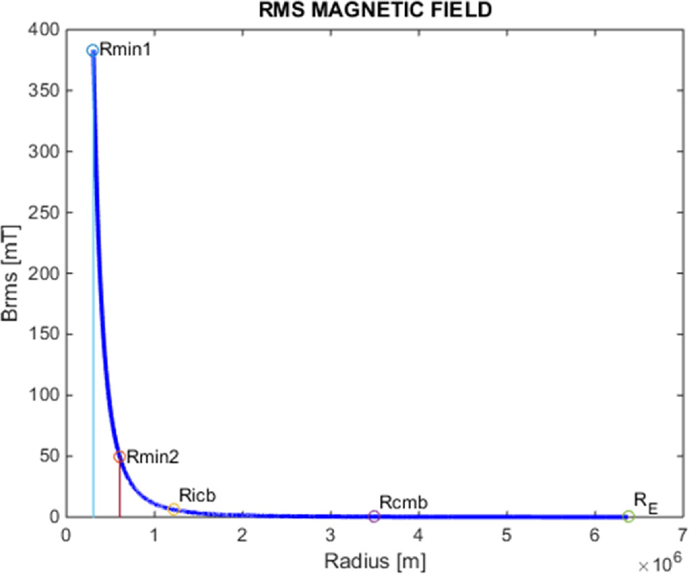
What could be the next step? If the existing computational models such as [8] and all relevant results were available, we could proceed to a post-processing to determine the unknown distribution of the RMS field intensity $B\left(r\right)$ in terms of the radius $r.$ We recognize that the primary concern of those pioneering investigators was to develop their multi-physics model from scratch and probably to perform a sort of sensitivity analysis regarding the most influencing parameters and their dependencies, a difficult task which does not allow focusing on details. The imposition of the boundary conditions in a Computational Fluid Dynamics (CFD) model is of major importance. As far as one can understand from reading, Neumann conditions of heat flux have been imposed while today it would be possible to directly impose the particular value of the field intensity $B(x,y,z)$ at every nodal point on the boundary (usually the CMB), simply implementing a computer software such as [41]. Not only that, but it becomes imperative to generate a structured computational mesh which will follow spherical surfaces of a specified radial step ${\rm{\Delta }}r.$ Then, taking the nodal points or/and the centroids on the spherical surface (face of these 'finite elements' or 'finite volumes') it would possible to perform post-processing and calculate the RMS value of the field intensity, $B\left(r\right),$ at each radius $r$ within the interval ${R}_{{ICB}}=1216\,{\rm{km}}\leqslant r\leqslant {R}_{{CMB}}=3486\,{\rm{km}},$ through the formula:

$$\begin{eqnarray}&&B(r)=\sqrt{\displaystyle \frac{\displaystyle \iint {\left[B(r,\phi ,\lambda )\right]}^{2}{r}^{2}\,\cos \,\phi \,d\phi \,d\lambda }{4\pi {r}^{2}}}\end{eqnarray} \tag{ 53 }$$

This information is still missing and could be the topic of a cooperative research program implementing several independent computer codes. After the function $B\left(r\right)$ has been determined, we can proceed applying equation (48).

Therefore, since the above information has not been documented in any published report [7–11], the author had to rely on older resources such as [24] and [25] which estimate the totality of Earth's magnetic field energy between $9\times {10}^{20}\,{\rm{J}}$ and $7\times {10}^{21}\,{\rm{J}}.$ Moreover, a second resource for our study was the breakdown proposed in [8], which suggests that the energy in the inner core is (at maximum) the 10% of the energy within that in the liquid outer core (see equation (35)). Moreover, the energy in the exterior of the outer core (${{\rm{\sim }}}6.7\times {10}^{18}\,{\rm{J}}$ thus small compared to either of the aforementioned $9\times {10}^{20}\,{\rm{J}}$ or $7\times {10}^{21}\,{\rm{J}}$), is at maximum 1% of the total energy content.

But again, another theoretical problem arises. What about the distribution of the field inside the inner core? Based on current scientific understanding, it is believed that the magnetic intensity inside the Earth's inner core does not vary significantly from point to point. The inner core is a relatively homogeneous solid metallic sphere, primarily composed of iron and nickel. However, it is important to note that the inner core's magnetic field is still subject to ongoing scientific research, and the available data is limited. The inner core's magnetic field is primarily generated by the motion of the liquid outer core, which surrounds it. The complex dynamics of the outer core can influence the magnetic field generation, and this, in turn, may have some impact on the magnetic intensity within the inner core.

While there may be small variations in the inner core's magnetic field, the available evidence suggests that any spatial variations from point to point within the inner core are likely to be relatively minor. The inner core is generally considered to exhibit a stable magnetic field with consistent intensity. However, it is worth noting that obtaining direct measurements from the inner core is extremely challenging due to its inaccessibility. Most of our knowledge about the inner core's magnetic field comes from indirect observations and modeling techniques. As research continues and more data becomes available, our understanding of the inner core's magnetic field variations may evolve.

It is worthy to mention that the assumption of a uniform magnetic field in the inner core, in conjunction with the reported values of [30–50] mT at the ICB and 4 mT in the liquid outer core, leads to energy breakdown which does not fill the abovementioned criterion 1:10 proposed in [8] (in general leads to higher energy in the inner core). This is for reasons we can only hypothesize about. For example, there may be a jump of the field at the ICB so that the uniform value inside the inner core is smaller than what the ICB dictates. Another reason may be that the calculated value of 4 mT is small for several technical unknown reasons. But, again, it is of major importance to replicate older works regarding the computational models of the Earth's interior with imposing and/or testing the IGRF-13 field values which all of us assume and expect to be valid on the CMB as well.

To bridge the gap between the value 0.42 mT at the CMB and the stated values between 30 and 50 mT at the ICB, several scenarios (such as linear interpolant, inverse-power, exponential, logarithmic, and polynomial) were offered. The difficulty to be in favour of a certain scenario is due to the fact that we have to determine such a supposedly smooth function $B\left(r\right)$ that its RMS value according to equations (48) or (53) is near 4 mT while the energy ratios in the cores fulfils the criterion $\left({\lambda =U}_{{inner}}^{{core}}/{U}_{{outer}}^{{core}}\leqslant 0.1\right).$

While the abovementioned ratio 1:10, described by equation (35), depicts that the ICB has a field of about 6 mT, this figure is quite smaller than the reported region between 30 and 50 mT. In brief, the value of 6 mT is easily bridged by a concave curve which fulfils the condition 1:10 by equation (35), while the values 30 to 50 mT can be also bridged but with a convex curve which does not fulfil the condition 1:10 by equation (35).

If the primary concern of a reader is to calculate the total energy of Earth's magnetic field, he/she has the opportunity to deal with the energy associated to a bar magnet. From the didactic point of view, this is a fourth model (in addition to the dipole, inverse-cubic and the IGRF-13 standard) of a tiny bar magnet which is extended from the North to the South Pole (more accurately tilted at an angle of about 11° with respect to Earth's rotational axis). Actually, in such a virtual case, the 'interaction' energy is about ${W}_{12}{\rm{\approx }}-3\times {10}^{17},$ of which the absolute value is smaller even than the total energy in the infinite space excluding the Earth (∼8×10¹⁷ J), not even considering Earth's interior. Therefore, we have to consider the self-energies due to the poles. Another shortcoming of this idea is that the field at the poles (not at the center) would become enormous high, which is not a real fact. Having said this, an improvement to this idea is to introduce the concept of a right cylindrical bar magnet (i.e., long as the previous one but of a certain diameter $D$) in which the stored energy is proportional to the square of the magnetization and a non-dimensional geometric factor (aspect ratio) $q=d/D$ (see, Davis et al [6]). For magnetic poles separated by distance $d=2{R}_{E},$ for $q=1.8$ we obtain the desired magnitude of (∼8×10¹⁷ J), while for $q=15650$ we obtain (∼7.05×10²¹ J). The latter model refers to a long and adequately thin cylindrical bar magnet, but it includes the singularities involved by the magnetic poles and also leads to a very weak field at Earth's centre.

Final Remark: The reported RMS value of $4$ mT, is a crucial figure to characterize the averaged state of the outer core. With respect to other RMS values in physics (such as the voltage of alternating current), the difference is that in the latter case the integral is taken with respect to time while here it is taken with respect to the volume of the Earth (i.e., ${B}_{{rms}}=\sqrt{\frac{\int {B}^{2}{dV}}{\int {dV}}}$). But similarly to the alternating current, the harmonic dependence of the field with respect to the latitude $\theta$ (in the Central Dipole (CD) model) leads to the fact that the RMS value equals to the peak value divided by $\sqrt{2}$ (see, [26]). We should pay attention that in the IGRF model the ratio max-to-min is much higher.

To give an example, in the particular case of the CMB, the IGRF-based RMS value of the field intensity is $0.42{\rm{mT}}$ while for the Greenwich meridian plane the minimum and maximum values were found to be $0.16{\rm{mT}}$ and $0.72{\rm{mT}}$ (see, [26]), respectively, thus the ratio peak-to-RMS value equals to 1.75 (i.e., higher than the usual $\sqrt{2}{\rm{\approx }}1.41$). Furthermore, as shown in figure 8, the ratio becomes still larger.

In any case, the maximum value of the field is larger than the RMS value, so we must take care whether the reported values represent RMS values $\left({B}_{{rms}}=\sqrt{\frac{\int {B}^{2}{dV}}{\int {dV}}}\right).$ Again, this study has considered that the reported value of 4 mT has been considered as the RMS value for the entire outer core.

From the several models developed and compared toward the estimation of field intensity and energy content inside the Earth, it was concluded that any judgment requires at least a working assumption. In the lack of consensus, the Maxwell's Second Law (divergence Gauss's law of magnetism) was considered in conjunction with a uniform magnetization thus leading to a uniform magnetic field inside the inner core. Then, assuming no field jump between the ICB and the inner core, it was shown that the energy content of the latter is fully determined by the total field at the ICB. Moreover, since the root square mean (RMS) value of the total field intensity inside the liquid outer core has been previously estimated at 4 mT it was possible to check that the usually stated field between 30 and 50 mT at the ICB leads to such a large energy content within the inner core that is much more than the accepted value of 10% of that within the outer core. This finding is in contrast at least to one of the established pioneering MHD dynamo computational models. In the lack of data, it was assumed that the total field about 0.42 mT at the CMB could be easily bridged with a supposed value of 6 mT at the ICB through a concave curve thus ensuring that the energy of the inner core is no more than 10% of that within the outer core. Alternatively, large values such as 30 and 50 mT at the ICB could also be bridged with the 0.42 mT at the CMB through a convex curve, however then the condition of 10% is no more fulfilled. The findings of this work show that a detailed post-processing of the computational results in the MHD dynamo model is imperative to establish the radial variation of the total RMS magnetic field at least between the ICB and CMB. Moreover, the variation of the total field inside the inner core is of great importance as well.

The data cannot be made publicly available upon publication because no suitable repository exists for hosting data in this field of study. The data that support the findings of this study are available upon reasonable request from the authors.

We consider the function

$$\begin{eqnarray}&&{B}_{CD}^{rms}(r)=\displaystyle \frac{\sqrt{2}{\mu }_{0}M}{4\pi {r}^{3}},0\lt r\lt \infty ,\end{eqnarray} \tag{ A-1 }$$

which expresses the RMS field intensity over any sphere of radius ${r}$ and centre ${O}$ (see, equation (40)). The aforementioned sphere may be either interior or exterior to the Earth, but in any case, should be concentric to the Earth. Select any point ${P}{(}{r}{=}{{R}}_{{P}}{,}{{B}}_{{{CD}}}^{{{rms}}}{)}$ on this curve and calculate (i) the field ${{B}}_{{{CD}}}^{{{rms}}}{(}{{R}}_{{P}}{)}$ according to equation (A-1) and (ii) the trapped energy ${{W}}_{{r}{\gt }{{R}}_{{P}}}$ outside the spherical surface ${(}{O}{,}{{R}}_{{P}}{)}$ according to the extension of equation (13b):

$$\begin{eqnarray}&&{W}_{r\gt {R}_{P}}^{rms}=\displaystyle \frac{{\mu }_{0}{M}^{2}}{12\pi {R}_{P}^{3}},\end{eqnarray} \tag{ A-2 }$$

Then we assume a uniform field of value ${{B}}_{{{uniform}}}^{{{rms}}}{(}{{R}}_{{P}}{)}$ in the interior of the whole sphere ${(}{O}{,}{{R}}_{{P}}{)}.$

Show that the energy due to the uniform field in the interior of the sphere ${(}{O}{,}{{R}}_{{P}}{)}$ equals to the energy due to the dipole variation (A-1) in the exterior of the same sphere ${(}{O}{,}{{R}}_{{P}}{)}.$

Appendix. Proof

According to equations (3) or (19), the energy in the interior of the sphere ${(}{O}{,}{{R}}_{{P}}{)}$ is given by the integral $\int {(}{{B}}^{{2}}/{2}{{\mu }}_{{0}}{d}{\upsilon }{)}$ over the volume surrounded by the sphere, which due to the assumption ${B}{=}{{const}}{.}$ simplifies to:

$$\begin{eqnarray}&&{\left({W}_{r\lt {R}_{P}}^{rms}\right)}_{uniform}=\displaystyle \frac{{B}^{2}}{2{\mu }_{0}}V=\displaystyle \frac{1}{2{\mu }_{0}}{\left(\displaystyle \frac{\sqrt{2}{\mu }_{0}M}{4\pi {r}^{3}}\right)}^{2}\cdot \left(\displaystyle \frac{4}{3}\pi {R}_{P}^{3}\right)=\displaystyle \frac{{\mu }_{0}{M}^{2}}{12\pi {R}_{P}^{3}},\end{eqnarray} \tag{ A-3 }$$

Comparing (A-3) with equation (A-2) we obtain the desired equality:

$$\begin{eqnarray}&&{\left({W}_{r\lt {R}_{P}}^{rms}\right)}_{uniform}={W}_{r\gt {R}_{P}}^{rms},\end{eqnarray} \tag{ A-4 }$$

Numerical application: For example, if the point $P$ is taken on Earth's surface, thus for ${M}{=}{7}{.}{6460}{\times }{{10}}^{{22}}$ ${{\rm{A}}}{{{\rm{m}}}}^{{2}}$ we have ${{B}}_{{E}}{=}\sqrt{{2}}{\mu }_{0}M/(4\pi {R}_{E}^{3})=4.2357\times {10}^{-5}$ T and the energy in the atmosphere will be ${{W}_{r\gt {R}_{E}}=W}_{{infinite}}={\mu }_{0}{M}^{2}/\left(12\pi /{R}_{E}^{3}\right)=7.7334\times {10}^{17}$ J. Moreover, considering the value of ${B}_{E}=4.2357\times {10}^{-5}$ T to be hypothetically uniform inside the entire Earth, the associated energy will be ${W}_{r\lt {R}_{E}}=\frac{{\left(4.2357\times {10}^{-5}\right)}^{2}}{\left(2{\mu }_{0}\right){\rm{\cdot }}{V}_{E}}=7.7334\times {10}^{17}{\rm{J}},{\rm{Q}}.{\rm{E}}.{\rm{D}}.\unicode{x0220e}$