

Abstract
The central purpose of this paper is extracting some novel and interesting soliton solutions of the extended (3+1)-dimensional Jimbo-Miwa equation(JME) which acts as an extension of the classic (3+1)-dimensional JME for the plasma and optics. First, we study the N-soltion solutions that is developed by the Hirota bilinear method (HBM). Then, the soliton molecules and Y-type soliton solutions are constructed via imposing the novel resonance conditions to the N-soltion solutions. In addition, we also explore the complex multiple soliton solutions via the HBM. The dynamic properties of the N-soltion, soliton molecules, Y-type soliton as well as the complex multiple soliton solutions are presented graphically. The developed soliton solutions of this research are all new and can enable us apprehend the nonlinear dynamic behaviors of the extended (3+1)-dimensional JME better.
Export citation and abstract BibTeX RIS
1. Introduction
As we all know, many problems in natural science can be expressed by the nonlinear partial differential equations (NPDEs), such as the heat conduction, chemical reaction, physics, soil moisture, hydrodynamics, vibration, nonlinear circuits and nonlinear optics, etc [1–12]. Considering the diversity of the NPDEs and the complexity of nonlinear problems, there is currently no method to obtain various solutions for all NPDEs. Therefore, the research on solving methods for the NPDEs remains a key and difficult topic in the field of nonlinear scientific research. So far, a good many effective and reliable approaches have emerged to deal with the NPDEs, for example the Darboux transformation approach [13–15], direct algebraic approach [16, 17], variational technique [18], Bäcklund transformation method [19–21], subequation method [22–24], tanh-function method [25, 26], exp-function approcah [27, 28], generalised exponential rational function approach [29, 30] and many others [31–38]. Under the current work, we are going to inquire into the extended (3+1)-dimensional JME that is given by [39]:

which is the extended form of the classic JME by Wazwaz. To get its Hirota bilinear equation(HBE), we make use of the following transformation:

where  Then we get the HBE as:


And there are:

Some outstanding performance achievements have been reached for equation (1.1). In [44], the resonant multi-soliton solutions are explored by using the linear superposition principle. In [45], some new periodic solitary wave solutions are studied. In [46], some new types of the rogue waves solutions are reported. In [47], some new exact solutions like the lump, lump-kink, and other interaction solutions are investigated. Hereby, we will extract some new and interesting soliton solutions such as the soliton molecules (SMs), Y-type soliton and complex multiple soliton solutions for equation (1.1).
The remaining content of this paper is arranged as: section 2 discusses the N-soliton solutions and extracts the SMs by applying the resonance conditions. Section 3 constructs the Y-type soliton solutions via imposing the corresponding resonance conditions. Section 4 looks into the complex N-soliton solutions. Finally, section 5 presents the conclusion.
2. The soliton molecules
By the HBE, the N-soliton solutions to equation (1.1) can be constructed as:

where

with

where 

 and
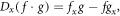
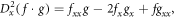
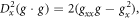
and  are non-zero constants,
  is the real constant.

and


For  we can get the 2-soltion solution as:

which is under equations (2.3), (2.4) and (2.5).
If the parameters are choosen as:
we illustrate the dynamics of the 2-soltion solution equation (2.6) on the interval ![$x,y\in \left[-\mathrm{10,10}\right]$](https://content.cld.iop.org/journals/1402-4896/99/1/015254/revision2/psad16fdieqn9.gif) in figure 1 for z = 0, t = 0, where (a) and (b) denote the 3-D plot and 2-D density respectively. It can be seen that the profile is formed by two kink soltions.
in figure 1 for z = 0, t = 0, where (a) and (b) denote the 3-D plot and 2-D density respectively. It can be seen that the profile is formed by two kink soltions.

Figure 1. Dynamic characteristics of the 2-soltion solution equation (2.6), (a) for the 3-D plot, (b) for the 2-D density.
Download figure:
Standard image High-resolution imageFor N = 3, we can get the 3-soltion solution as:


which is under equations (2.3), (2.4) and (2.5).
If the parameters are assigned as:

we plot the dynamics of the 3-soltion solution equation (2.7) on the interval ![$x,y\in \left[-\mathrm{10,10}\right]$](https://content.cld.iop.org/journals/1402-4896/99/1/015254/revision2/psad16fdieqn10.gif) in figure 2 at z = 0, t = 0. Here we can see that the profile is stacked and interlaced by three kink soltions.
in figure 2 at z = 0, t = 0. Here we can see that the profile is stacked and interlaced by three kink soltions.
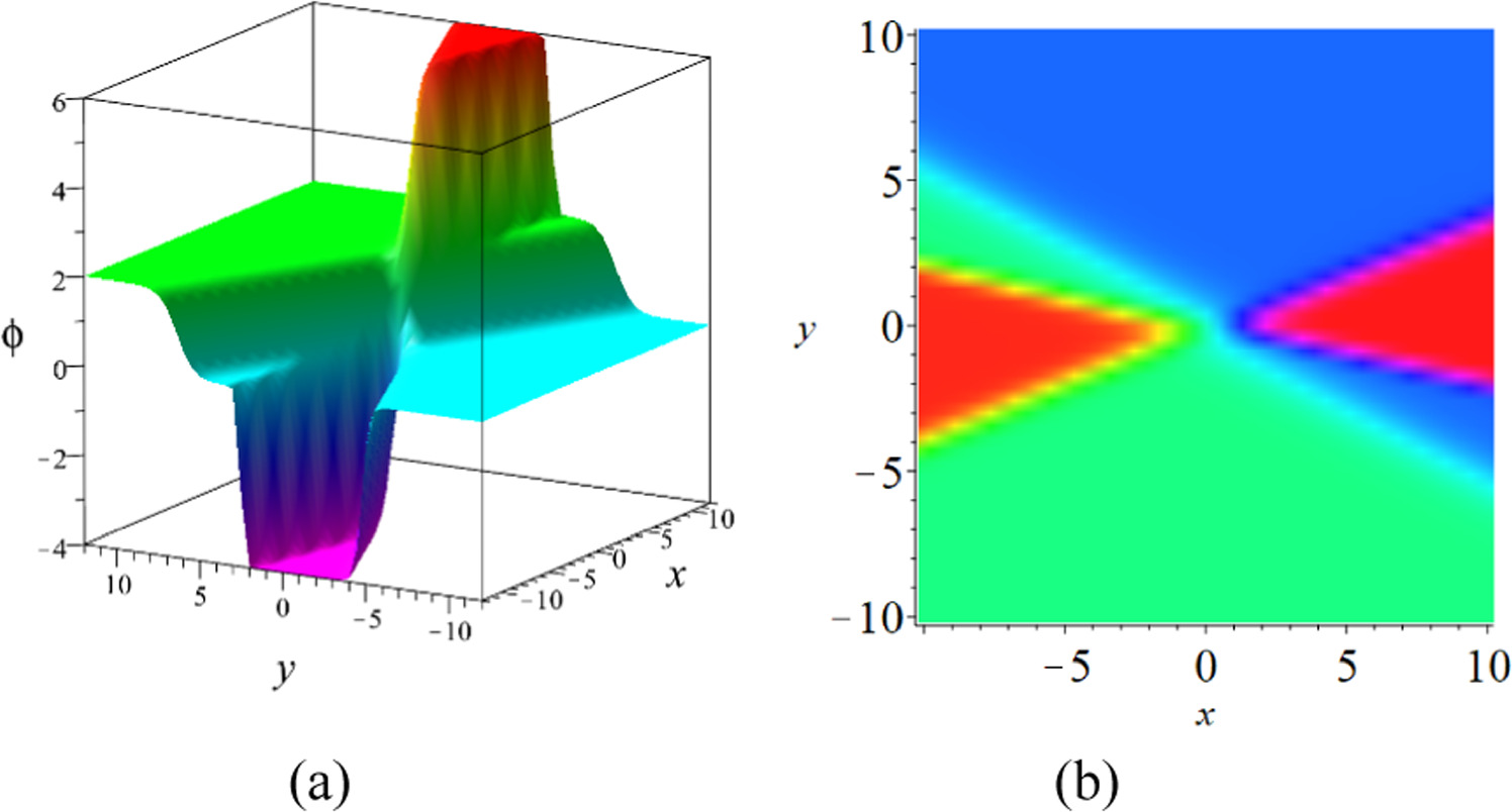
Figure 2. Dynamic characteristics of the 3-soltion solution equation (2.7) (a) for the 3-D plot, (b) for the 2-D density.
Download figure:
Standard image High-resolution imageRecently, the SMs are the research hotspots [48–51]. To get the SMs, we apply the following resonance conditions [52–55]:
Case 1: On the (x, y)-plane, the resonance condition is:

Thus we have:

We can get the SMs on the (x, y)-plane by inserting equation (2.9) into equations (2.1) and (2.2).
Case 2: On the (x, z)-plane, the resonance condition is:

Thus we have:

So we can find the SMs on the (x, z)-plane with above results.
Case 3: On the (y, z)-plane, the resonance condition is:

Thus we have:

Similarly, the SMs on the (y, z)-plane can be obtained by taking above results into equations (2.1) and (2.2).
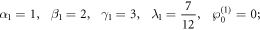
If we select the parameters as:

the characteristics of the soliton molecule with 2 soltions on the (x, y) plane are presented in figure 3 for the different times. By our our careful observation, it can be found that the two solitons are parallel to each other.
Figure 3. Dynamic characteristics of the soliton molecule with 2 solitons equation (2.6) on the (x, y) plane, (a), (d) for t = 1, (b), (e) for t = 2, (c), (f) for t = 3.
Download figure:
Standard image High-resolution imageIf we use the parameters as:


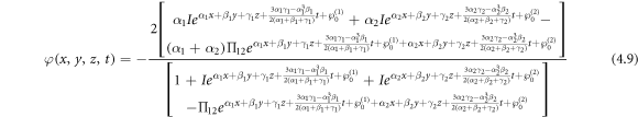
 the performances of the soliton molecule with 3 soltions on the interval
 ![$x,y\in \left[-\mathrm{20,20}\right]$](https://content.cld.iop.org/journals/1402-4896/99/1/015254/revision2/psad16fdieqn14.gif) are described in figure 4. Obviously, it is can seen that the 3 solitons are the kink solitons and are parallel to each other.
are described in figure 4. Obviously, it is can seen that the 3 solitons are the kink solitons and are parallel to each other.

Figure 4. Dynamic characteristics of the soliton molecule with 3 solitons equation (2.7) on the (x, y) plane, (a), (d) for t = 1, (b), (e) for t = 2, (c), (f) for t = 3.
Download figure:
Standard image High-resolution imageThrough the careful observation the From figures 3 and 4, it finds the characteristic for the SMs is the solitons in the soliton molecules remain parallel and advance at the same speed, and the solitons never intersect.
3. The Y-type soliton solutions
To find the Y-type soliton solutions, we can adopt the following resonance conditions to the N-soliton solutions [54, 56–60]:


Solving it yields:

which is the resonance Y-type soliton solution condition.
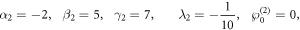
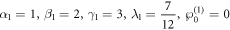
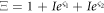
For  if the parameters are selected as:

then we depict the fusion phenomenon of the Y-type soliton through the 3-D plot and 2-D density on the illustrate ![$x,y\in \left[-\mathrm{20,20}\right]$](https://content.cld.iop.org/journals/1402-4896/99/1/015254/revision2/psad16fdieqn16.gif) at the different time for z = 0 in figure 5, which indicates that the interaction between the fusion of the resonant Y-shaped solitons is elastic.
at the different time for z = 0 in figure 5, which indicates that the interaction between the fusion of the resonant Y-shaped solitons is elastic.

Figure 5. Dynamic characteristics of the Y-type soliton equation (2.6), (a), (d) for t = 0, (b), (e) for t = 5, (c), (f) for t = 10.
Download figure:
Standard image High-resolution imageWhen  we can extract the expression of the two 2-resonance Y-type solution as:


If we choose the parameters as:


the legend of the 2-resonance Y-type solitons at different time for z = 0 is presented in figure 6. Here it indicates that the waveform are formed by two fission resonance waves, and the interaction of the 2-resonance Y-type soliton is elastic.
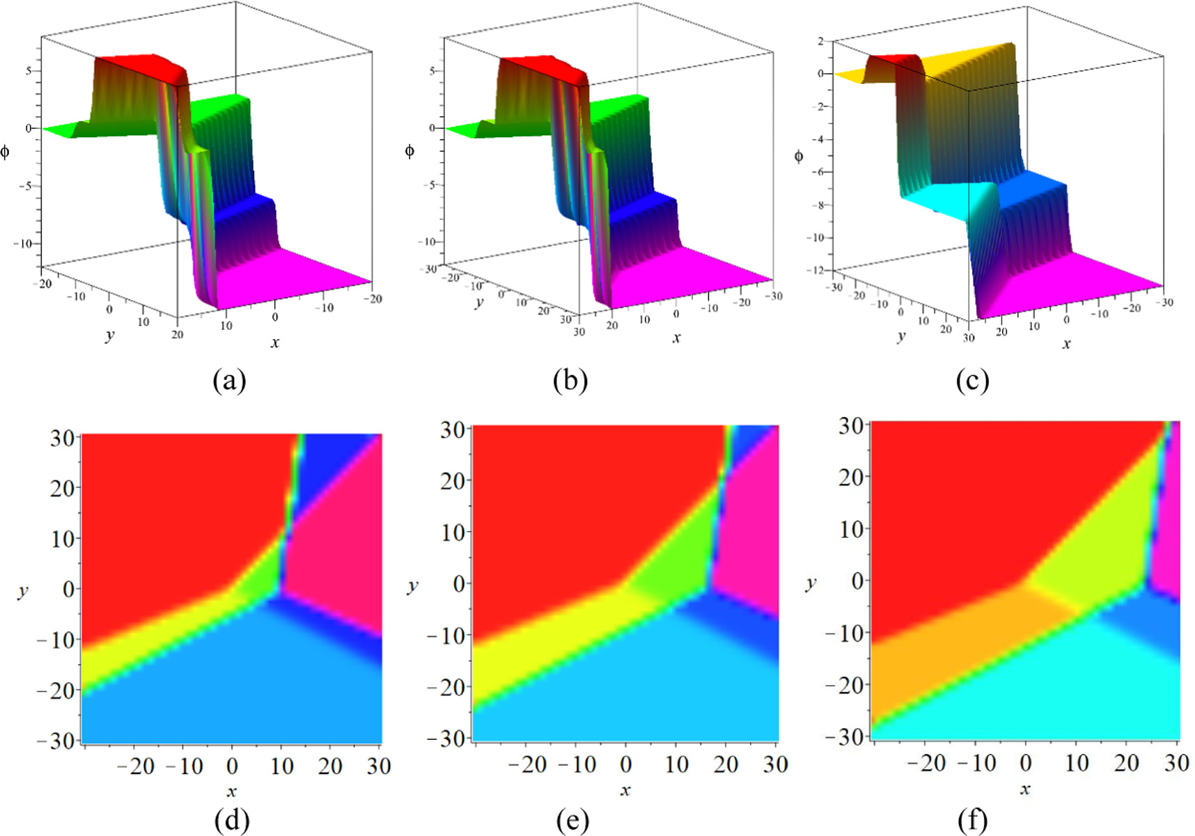
Figure 6. Dynamic characteristics of the 2-resonance Y-type solitons equation (3.3), (a), (d) for t = 0.4, (b), (e) for t = 0.7, (c), (f) for t = 1.
Download figure:
Standard image High-resolution image4. The complex multiple soliton solutions
This section is going to construct the complex multiple soliton solutions. Now we assume the complex one soltion solution as:

with

Putting them into equation (1.5), we have:

Thus, we can find the complex one soliton solution of equation (1.1) is acquired:

We can develop the complex two soliton solution with the form as:

with

Taking equations (4.5) and (4.6) into equation (1.3), we have:


Then the complex two soliton solution can be obtained as:
Similarly, we can develop the complex three soliton solution as:

where


Then, taking equations (4.10), (4.11) and (4.12) into equation (1.3), the complex 3-soliton solutions can be obtained. This reveals that the complex multiple soliton solutions can be found by using the same operation in the general form as:

with


If the parameter values are used as:
we draw the profiles of the absolute value of the complex one soliton solution for z = 0 and t = 0 on the interval ![$x,y\in \left[-\mathrm{10,10}\right]$](https://content.cld.iop.org/journals/1402-4896/99/1/015254/revision2/psad16fdieqn19.gif) in figure 7, where figures 7(a) and (b) stand for the 3-D plot and 2-D density respectively. Here we can see that the wave is the kink soliton.
in figure 7, where figures 7(a) and (b) stand for the 3-D plot and 2-D density respectively. Here we can see that the wave is the kink soliton.

Figure 7. Dynamic characteristics of the absolute value of the complex one soliton solution equation (4.4) for z = 0 and t = 0.
Download figure:
Standard image High-resolution imageIf the parameter values are selected as:
the dynamic characteristics of the absolute value of the complex two soliton solution for z = 0 and t = 0 is illustrated in figure 8. The interval is selected as ![$x,y\in \left[-10,\,10\right].$](https://content.cld.iop.org/journals/1402-4896/99/1/015254/revision2/psad16fdieqn20.gif) Here it finds that the waveform is the interreaction of two kink solitons.
Here it finds that the waveform is the interreaction of two kink solitons.
Figure 8. Dynamic characteristics of the absolute value of the complex two soliton solution equation (4.9) for z = 0 and t = 0.
Download figure:
Standard image High-resolution imageIf the parameters are chosen as:


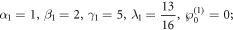
Figure 9 illustrates the dynamic characteristics of the absolute value of the complex three soliton solution for z = 0 and t = 0. It's obvious that the outline is formed by three kink solitons intersecting with each other.

Figure 9. Dynamic characteristics of the absolute value of the complex three soliton solution equation (4.10) for z = 0 and t = 0.
Download figure:
Standard image High-resolution image
5. Conclusion
In this research, we have constructed some novel and interesting soliton solutions of the new extended (3+1)-dimensional JME. By imposing some resonance conditions to the N-soliton solutions, we developed the soliton molecules and Y-type soliton solutions. Additionally. we also explored the complex multiple soliton solutions by taking advantage of the HBM. The dynamical characteristics of the attained soliton solutions are described graphically by applying the reasonable parameters. The derived outcomes in this study are all new, which can be used to expand the range of exact solutions to the (3+1)-dimensional JME and can help us better understand and master its physical properties.
Data availability statement
The data cannot be made publicly available upon publication because they contain sensitive personal information. The data that support the findings of this study are available upon reasonable request from the authors.
Funding
This work was supported by the Key Programs of Universities in Henan Province of China (22A140006), Program of Henan Polytechnic University (B2018–40).
Conflict of interest statement
This work does not have any conflicts of interest.