

Abstract
This paper exposes the theoretical and microcontroller implementation probing of the piecewise nonlinear resistor-capacitor shunted Josephson junction circuit (PNRCSJJC). The PNRCSJJC is characterized by no steady state when the applied current is greater than one and exhibits two steady states in which one is a focus and its counterpart a saddle-node for excitation current less than or equal to one with credit to the Routh–Hurwitz criterion. The PNRCSJJC exhibits periodic characteristics, quasi-periodic characteristics, varying structures of chaotic characteristics, and coexisting behaviors which is proved qualitatively by the microcontroller execution method. The polarity of the chaotic signal in the voltage state variable is flexibly altered by varying a constant parameter included in the rate equations of PNRCSJJC.
Export citation and abstract BibTeX RIS
1. Introduction
The JJ has heavily been underlined by increasing noise phenomena and complex characteristics as a consequence of its non-linear entanglement [1]. The junction adheres to quantum norms as it violates classical assumptions [2]. This notion redirected interest toward the junction concerning complex models and chaos [3–10]. These concerns and explorations have been achieved both experimentally and theoretically [11, 12]. The perfect dynamics exposed by the JJ resulted in associating the junction with different applications such as: digital logic cryogenic [13], metrology measurements [14], spin-filters [15], parametric amplifiers [16], voltage standards [17], actuators [18], magnetometers [19], highly responsive SQUID detectors [20], microwave sensors [21], coded communication and encryption [22, 23], and others.
The state-of-the-art regarding various nonlinearities when considering the JJ after its discovery thanks to Josephson [24], was the different models reported. The traditional model involved the resistors, the JJ element, and the capacitor connected in parallel to which an applied current is used for excitation (RCSJJ model) and afterward, the updated model to which the shunted loop consisting of an inductor is added parallelly to the RCSJJ model (RCLSJJ model) also referred to as the JJ jerk oscillator. In its earlier literature, the majority of the models considered the linear case where all the components of the JJ were linear. In its recent literature, the considered models are nonlinear where the nonlinear RCSJJ and RCLSJJ have been investigated. It's of high importance to expose that in the case any of the components are nonlinear, the said model is referred to as the nonlinear model. The nonlinearities are not limited to the components of the JJ models, but also to the nature of the superconducting materials. In this consideration, high-temperature [25] and low-temperature [26] superconducting materials, superconducting materials with high density [27], topological superconducting materials [28], and others have been established.
In this research inquiry, the resistance of the resistor across the JJ is considered nonlinear. In its earlier and wider literature, the JJ models investigated considered the resistor with constant resistance [23, 29–32]. Other aspects of the nonlinear resistance in the JJ models include fractal resistance [33, 34] and smooth irregular resistance [35]. Increasing attention to the junction resulted in the modified nonlinear models with the resistance of the shunted resistor inversely proportional to the JJ voltage resulting in quadratic damping (referred to as quadratic RCSJJ or RCLSJJ) in the models [36, 37]. Quadratic characteristics of the damping resulted in a complex response, metastable states, and instability of the model when radiofrequency driving was observed [38, 39]. This consideration was reformulated by employing the Hamiltonian method [40]. Also via the Melnikov technique, a minimum threshold for complex characteristics was predicted therein [37]. Other considerations of the nonlinear resistance were investigated among which the fractal resistance was studied. Here, Kruchinin et al [33] studied a generator of chaotic behaviors with a focus on the JJ model with a fractal resistive subgap. Also in 2008, they presented a JJ model with an insulating layer possessing radioisotopes which in essence is the contribution of the fractal resistance [41]. They observed the emission of  –particles by radioisotope which contributed to the non-equilibrium dispersive behaviors of composite materials, and lastly, they studied the distribution of the different dynamics in a non-equilibrium fractal JJ. With major concern in encryption and technology, the dynamics of fractal resistance in tunneling JJ was reported in [42]. In essence, the circuit model, contribution of forced parameters, and fractal resistance to the dynamics of the JJ were evaluated. Further, Sakai and Yamaguchi [43] numerically evaluated bifurcations and transitions to chaos in the smooth nonlinear resistor and capacitor shunted JJ (SNRCSJJ) circuit stimulated by an AC source. Bartuccelli et al [37] investigated chaos in the SNRCSJJ circuit stimulated by an AC source analytically by employing the Melnikov function method. Yao [44] via numerical simulations revealed bifurcation, phase-locking, and chaos in the SNRCSJJ circuit driven by AC through diagrams. Recently in [35], the authors reported hysteresis phenomenon, periodic behaviors, relaxation behaviors, chaotic behaviors, bistable periodic attractors, and coexisting attractors in the SNRCSJJ via numerical analysis. Ambika [45] exploited the model of nonlinear resistance while considering the DC and AC stimulations and exposed crisis as the main criteria for the onset of complex behaviors. For distinct parameters of the driving force, they reported period doubling preceded by interior complex behaviors. With the observed chaotic behaviors, their model shuttled irregularly between various unstable voltage steps. In these highlighted considerations, the mechanism, structures, and nature of chaos are highly absent and the lacuna is filled by this research paper. This model of nonlinear resistance has been absent in the recent literature of the JJ. Comparing the above-exposed dynamics in Ambika's [45] model with the ones reported in this research paper, novel characteristics have been achieved including periodic characteristics, quasi-periodic characteristics, varying structures of chaotic characteristics, and coexisting behaviors which is proved qualitatively by the microcontroller execution method, and lastly, the offset boosting mechanism in which the polarity of the chaotic signal in the voltage state variable is flexibly altered by varying a constant parameter included in the rate equations of PNRCSJJC. The concern of offset boosting control is in signal conditioning and the redesigned of complex behaviors from bipolar to equivalent unipolar ones which find practical and experimental applications regarding the displacement of complex behaviors in coordinate phases. Hence, the importance of signal conditioning and redesigning cannot be overlooked as it is associated with varieties of techniques among which are time-reversible symmetry [46], repellor construction [47], conditional symmetry [48], attractor selfreproducing [49], and attractor doubling [50]. Recently, Wang et al [51] observed experimental hidden Chua's attractor. In their consideration, offset control was employed to redesign the attraction basin and mapping the non-zero initial values to zero ones. Hence, the attraction basin was intersected with the origin, permitting them to experimentally observe the hidden attractor by means of pre-discharging all dynamic elements. Also, Xu et al [52] exposed multiple attractors in their proposed memristive Chua's circuit. They obtained and proved their dynamics via numerical simulations, hardware circuit experiments, and PSIM circuit simulations. Theoretically, they obtained two stable nonzero saddle-foci and their model exhibited the unusual and striking dynamical behavior of multiple attractors with multistability. The new interesting dynamical behaviors, experimental validation of the numerical results, and finally offset boosting mechanism in this paper are new regarding the considered model and will also contribute in adding the literature of the nonlinear resistance in JJ models comparable to the exposed literature.
From this exposure, this paper aims to examine the theoretical and microcontroller execution probing of the PNRCSJJC. This consideration fills the lacuna and adding to the literature of this scare exploited model of the JJ are the major contributions. The paper follows the following format: The theoretical probing in the preceding sub-part, the microcontroller implementation of the PNRCSJJC in section 3, and the conclusion in section 4.
2. Theoretical probing of PNRCSJJC
Figure 1 presents the piecewise nonlinear Josephson junction circuits under investigation.

Figure 1. Representation of the PNRCSJJC.
Download figure:
Standard image High-resolution imageFigure 1 is a parallel combination of the capacitor  the JJ current
  and the nonlinear resistor
  stimulated by the applied current
  The piecewise nonlinear resistor
  is defined as
  where
where  is the voltage across the JJ and
  is a constant parameter [41]. By carrying out Kirchhoff's laws in figure 1, system (1) is obtained:


with the time given by  JJ critical current
  phase difference
  Planck's constant
  and
and  the electronic charge. The dimensionless system (1) is given by:


with 

 and
and  The applied current can be considered as a direct current (DC):
  or an alternative current (AC):
  where
where  are DC, modulation current, and modulation pulsation, respectively. For
  system (2) has two steady states:
  and
and  while for
  system (2) has no-steady state. The characteristic polynomials related to
  are given by:

The steady state  is saddle because
  and
and  The steady state
  is a focus because
  with
with 
When the applied current is an AC ( ), the two parameters' greatest Lyapunov exponent (GLE) diagrams are depicted in figures 2 and 3.
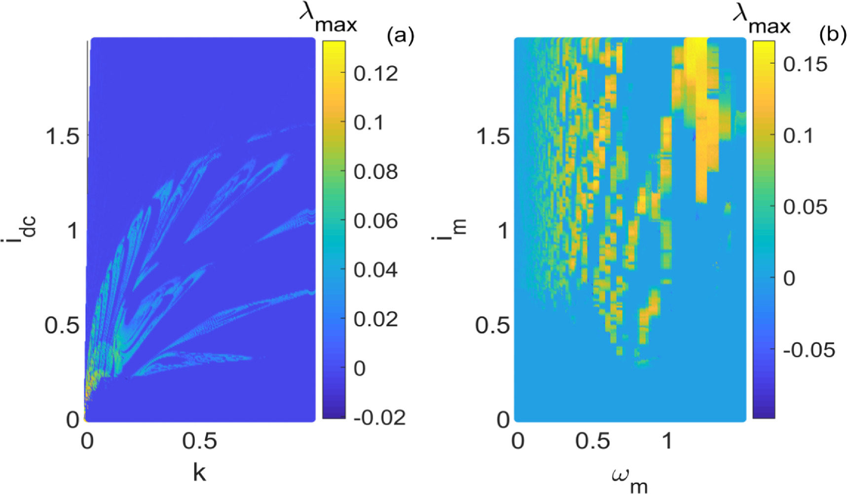
Figure 2. Dynamical behavior maps of PNRCSJJC in (a) space for
 and (b)
  space for
 .
.
Download figure:
Standard image High-resolution image
Figure 3. Dynamical behavior maps of PNRCSJJC in (a) space for
 and (b)
  space for
 .
.
Download figure:
Standard image High-resolution imageFigure 2 shows the GLE obtained by varying simultaneously  and
and  as shown in figure 2(a) and
  and
and  as shown in figure 2(b). Irregular behaviors are obtained when
  and regular characteristics for
Similarly, figure 3 shows the GLE obtained by varying concurrently  and
and  as represented in figure 3(a) and
  and
and  as shown in figure 3(b). Chaotic characteristics are obtained when
  and regular behaviors for
  It is important to highlight that varying the planes as much as the system parameters greatly influences massively the rich dynamical characteristics appearing in PNRCSJJC. The bifurcation plot and the related GLE versus
  are established in figure 4 for distinct values of the parameters


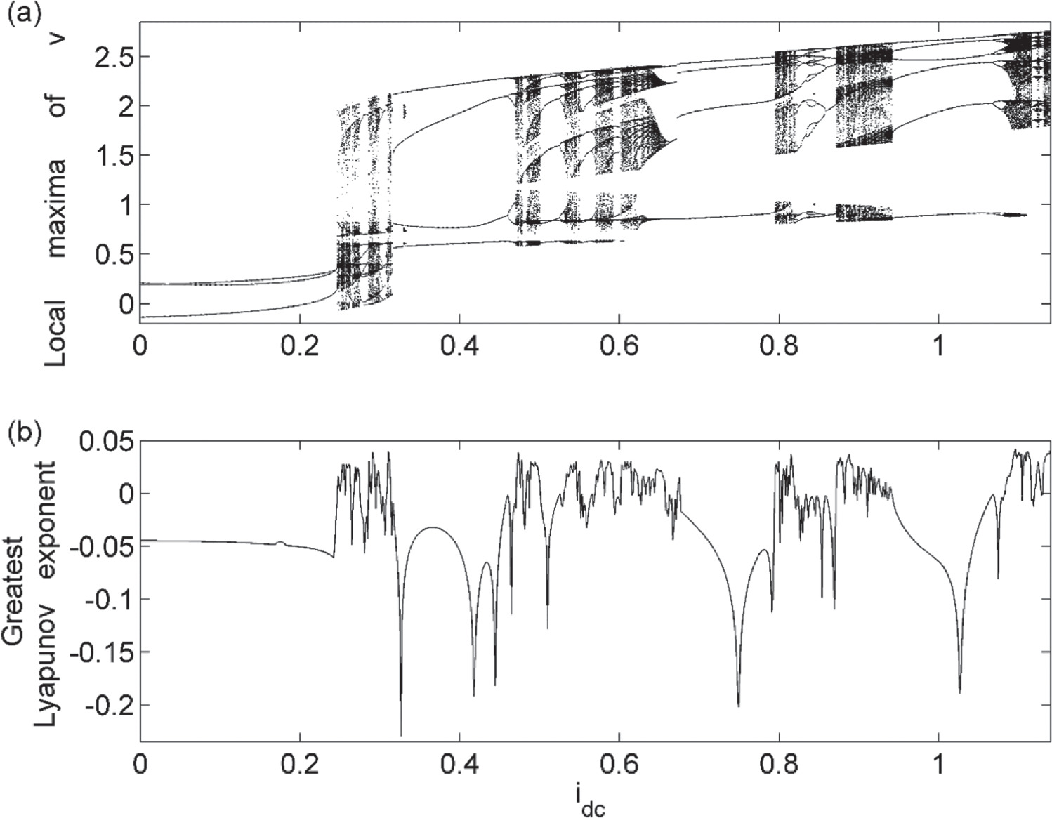
Figure 4. Bifurcation plot of  (a) and the corresponding GLE (b) versus
  for
for 
 and
and  .
.
Download figure:
Standard image High-resolution imageThe bifurcation plot of  of the PNRCSJJC against
  exposes period doubling attractor to complex attractors, and interception between complex and regular attractors as shown in figure 4(a) which is proved by the GLE established by figure 4(b). The bifurcation plot and the related GLE versus
  are depicted in figure 5 for distinct values of the parameters


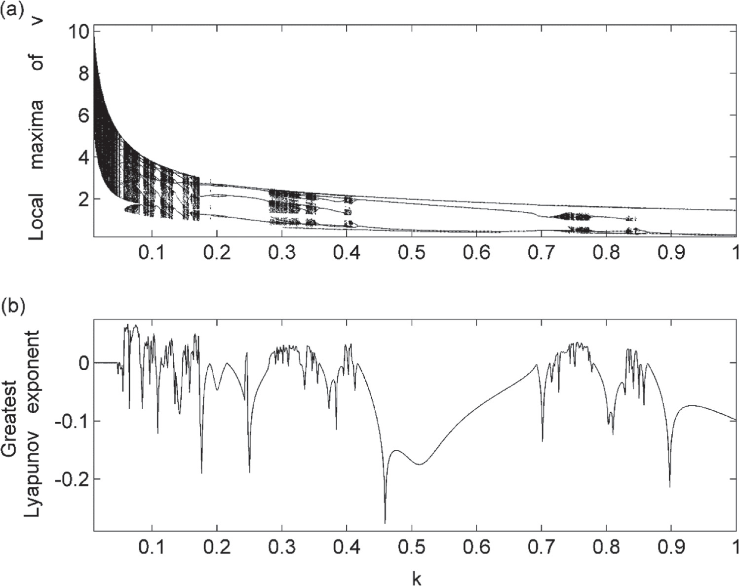
Figure 5. Bifurcation plot of  (a) and the corresponding GLE (b) against
  for
for 
 and
and  .
.
Download figure:
Standard image High-resolution imageThe evolution of the local maxima of  of the PNRCSJJC against
  with step size 0.001 exposes quasi-periodic oscillations, chaos, interception between chaos and regular attractors, and finally period doubling attractor as shown in figure 5(a) which is proved by the GLE established by figure 5(b). The local maxima of v and the related GLE versus
  are illustrated in figure 6 for distinct values of the parameters


Figure 6. Bifurcation plot of  (a) and the corresponding GLE (b) against
  for
for 
 and
and  .
.
Download figure:
Standard image High-resolution imageThe evolution of the local maxima of v of the PNRCSJJC against  with step size 0.001 exposes quasi-periodic oscillations, chaos, interception between chaos and regular attractors, and finally, limit circle as established in figure 6(a) which is proved by the GLE in figure 6(b). The bifurcation plot and the related GLE versus
  are illustrated in figure 7 for distinct values of the parameters


Figure 7. Bifurcation plot of  (a) and the corresponding GLE (b) versus
  for
for 
 and
and  Varying
  in ascending and descending order gives the black and red plots, respectively.
Download figure:
Standard image High-resolution imageThe evolution of the local maxima of  of the PNRCSJJC against
  with step size 0.001 exposes limit circle to period doubling attractor, coexisting behaviors, monostable complex attractors, and interception between complex and regular attractors as in figure 7(a) which is proved by the GLE established by figure 7(b). Dynamical characteristics revealed in figures 4 to 7 are illustrated in figure 8.

Figure 8. Phase projections in  plane for distinct values of the parameters


 (a)
(a) 


 (b)
(b) 


 (c)
(c) 


 (d)
(d) 


 (e)
(e) 


 (f)
(f) 


 (g)
(g) 


 (h)
(h) 


 (i)
(i) 


 (j)
(j) 


 and (k1, k2)


 The curves in black are obtained by using the initial conditions
  while the curves in red are obtained by using the initial conditions
  .
.
Download figure:
Standard image High-resolution imageFigure 8 is characterized by vast distinct chaotic behaviors in figures 8(a)–(j) and coexisting attractors in figures 8(k1 and k2) about the plane  The interest of the considered plane is a consequence of the phase turning to infinity with time and to bring it into the real regime, the cosine function of the phase is plotted. The coexisting characteristics shown in figure 8 are further elaborated by the basin of attraction in figure 9.

Figure 9. Basin of attraction of the PNRCSJJC in  plane for

 and
and  .
.
Download figure:
Standard image High-resolution imageThe coexisting characteristics achieved in the PNRCSJJC for different initial states are affirmed by the basin of attraction in figure 9. Here, chaos is represented with initial states in blue shades while periodic behavior is represented with initial states specified in black domains. The GLE which is the discriminant is evaluated for each set of initial conditions and chaotic domains are obtained for  and periodic behaviors for
  The two incipient states are concomitantly varied with respective step sizes of 0.001 to include all dynamic points.
The state variable  appears twice in the system (2) describing the PNRCSJJ. So, system (2) experiences the offset boosting in
  By substituting
  by
by  where
where  is the boosting controller, system (2) becomes:


System (4) has no steady state for  and two steady states:
  and
and  for
for  Steady states
  are associated with the characteristic system (5):

The steady state  is a saddle node because
  and
and  while the steady state
  is a focus because
 with credit to the Routh-Hurwitz criteria. So, the stability exploration of
  do not depend on
  Figure 10 presents the phase portrait and the evolutions with time of the system (4) for specific values of the parameter

Figure 10. Phase portraits considering the plane  and the evolutions with time of
  for different values of
  plotted for system (4):
  (red),
  (black), and
  (magenta) for

 and
and  The starting states are
  .
.
Download figure:
Standard image High-resolution imageThe polarity of the complex signal  is flexibly changed by varying the parameter
  as depicted in figure 10.
3. Microcontroller execution probing of PNRCSJJC
The blueprint of the microcontroller execution of the PNRCSJJC is exposed in figure 11.
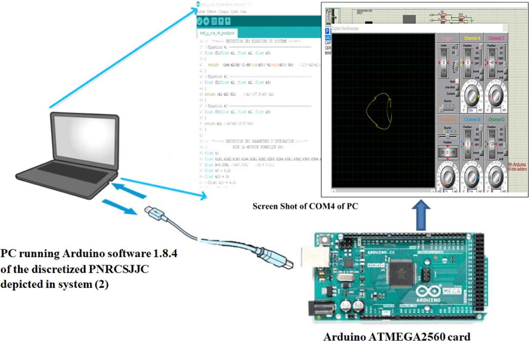
Figure 11. Blueprint of the microcontroller method.
Download figure:
Standard image High-resolution imageFigure 11 is constructed thanks to the ATMEGA2560 microprocessor. The ATMEGA2560, R-2R resistors set-up, the capacitors, the computer, digital oscilloscope are connected to constitute the experimental methods for the microcontroller execution of the PNRCSJJC as exposed in figure 11. With reference to the Runge–Kutta algorithm and Arduino software, system (2) is transformed and executed. The observation of the output equivalent analog signal on the screen of the digital oscilloscope terminates the implementation process. This scheme permits the comparison of results between numerical simulation and experimental results. The outputs are snapped and exposed in figures 12 and 13. For easy presentation, the first six chaotic characteristics of figures 8(a)–(f) reproduced by the microcontroller design in figure 11 of the PNRCSJJC are exposed in figure 12.
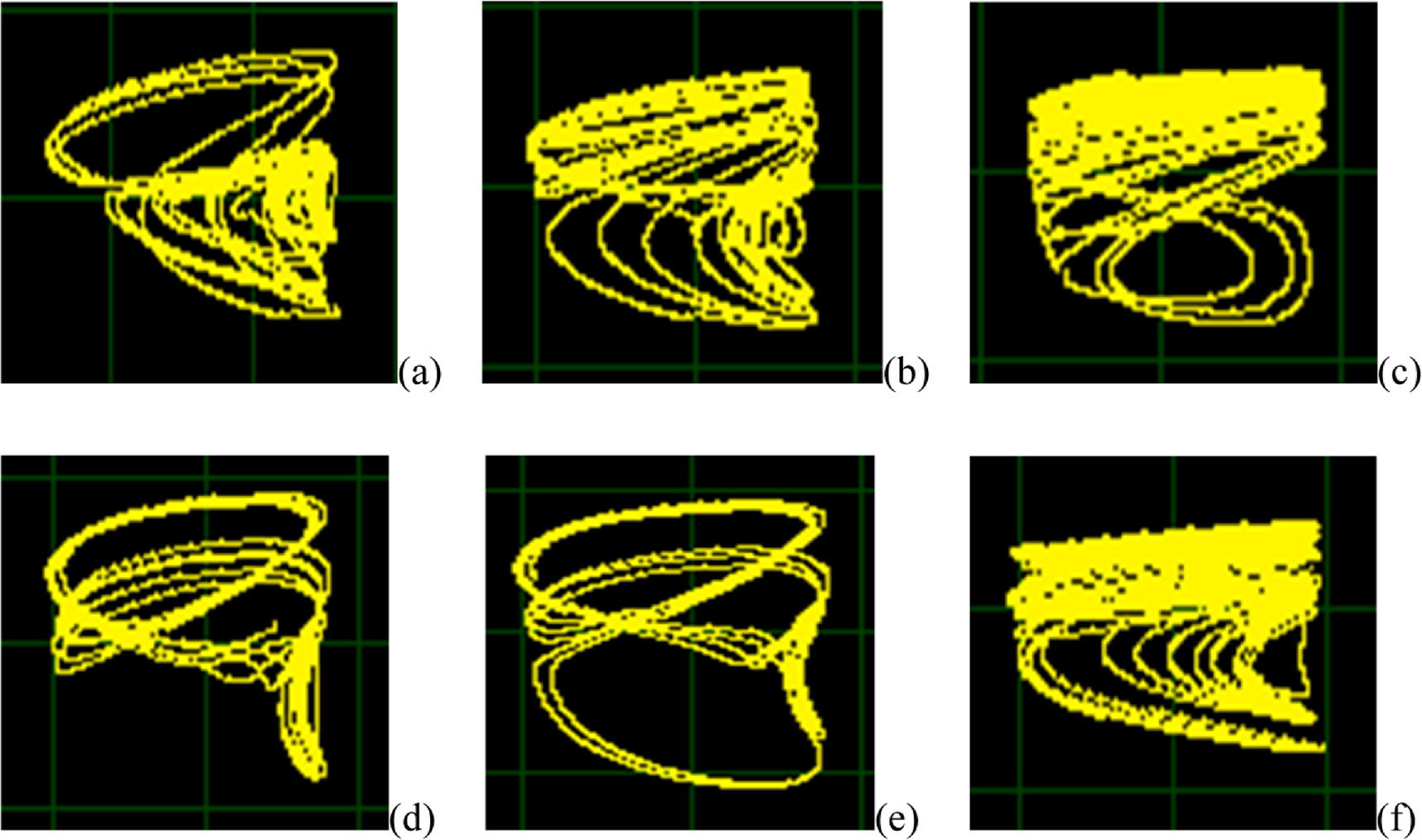
Figure 12. Microcontroller dynamics of the PNRCSJJC gotten with the same parameters as the ones in figures 8(a)–(f) in the same order.
Download figure:
Standard image High-resolution image
Figure 13. Microcontroller dynamics of the PNRCSJJC gotten with the same parameters as the ones in figures 8((g)–(j), k1, and k2) in the same order.
Download figure:
Standard image High-resolution image
The numerically simulated chaotic attractors of figures 8(a)–(f) find qualitative agreement with the microcontroller realization attractors of figures 12(a)–(f) achieved from figure 11. The parameters of figures 12(a)–(f) are as those in figures 8(a)–(f) respectively. Furthermore, chaotic attractors in figures 8(g)–(j) and the coexisting attractors exposed in figures 8(k1 and k2) are illustrated in figure 13.
The chaotic attractors of figures 8(g)–(j) and the coexisting attractors in figures 8(k1 and k2) obtained from the numerical simulation are proved by the microcontroller chaotic attractors in figures 13(g)–(j) and the microcontroller periodic and chaotic behaviors for the same parameters but distinct recipient states of figures 13(k1 and k2) respectively. The qualitative similarities between figures 8((g)–(j), k1, and k2) and figures 13 ((g)–(j), k1, and k2) respectively permit the validation and comparison of theoretical and experimental attractors. Comparatively to PSIM or OrCAD-PSpice, it can be highlighted that being programmable gives microcontrollers special concern and also referred to as 'special purpose computers', they execute specific programmed tasks stored in ROM. They are available with onboard memory and I/O ports which eradicate the construction of circuits possessing separate external RAM, ROM, and peripheral chips like PSIM or OrCAD-PSpice. They are readily available, cheap, and have low power consumption. These characteristics of the microcontroller make it a better choice for embedded applications compared to the OrCAD-PSpice or PSIM.
4. Conclusion
The theoretical and microcontroller realization probing of the piecewise nonlinear resistor-capacitor shunted Josephson junction circuit was investigated in this paper. When the applied current is greater than one, no steady state was reported in the piecewise nonlinear resistor-capacitor shunted Josephson junction circuit while two steady states with one a focus and its counterpart a saddle node for the applied current lesser than or equal to one with credit to Routh–Hurwitz criterion. The piecewise nonlinear resistor-capacitor shunted Josephson junction circuit exhibited periodic characteristics, quasi-periodic oscillations, varying structures of chaotic characteristics, and coexisting behaviors thanks to numerical simulations. The microcontroller method was used to prove the simulated results as qualitative similarities were put into view. Offset boosting was achieved in the voltage state variable. In this view, the polarity of the chaotic signal in the voltage state variable was flexibly altered by varying a constant parameter included in the rate equations of the piecewise nonlinear resistor-capacitor shunted Josephson junction circuit. The study of bursting mechanism generation can be done in the investigated model and intermittent phenomenon verified in future consideration. Also, other considerations like employing a function to understand offset boosting control will be interesting for future works.
Acknowledgments
This work is partially funded by the Center for Nonlinear Systems, Chennai Institute of Technology, India via funding number CIT/CNS/2023/RP-007.
Data availability statement
The data that support the findings of this study are available upon reasonable request from the authors.
Statements and declarations
Competing interest
The authors have no relevant financial or non-financial interests to disclose.