

Abstract
Nanofluids play a vital role in the improvement of our practical life. The potential usage of nanomaterials in different applications such as oil recovery, refrigeration systems, a freeze of electrical components in computers, development of liquid displays, cooling spirals, mechanical engineering, electrical engineering, heat storage devices and biotechnology. Swimming microorganisms have a crucial role in various areas of life, such as medicines, bioengineering, biofuels and food processing. Microorganisms are used as antibiotics in medicine and help to create a vaccine. Keeping in mind these applications, the current research provides a mathematical model for bioconvection Sutterby nanofluid flowing past the rotating stretching disk with magnetic field, motile microorganisms, chemical reactions and heat generation. The Brownian movement and thermophoresis diffusions are also considered. The governing equation structures are simplified by suitable transformations. A popular bvp4c solver in MATLAB computational software is employed to achieve numerical results for the non-linear model. The flow evaluation for the effects of several prominent numbers on temperature, velocities, concentration and motile microorganism profiles is executed graphically and numerically. The volumetric concentration of nanomaterial rises for thermophoresis number while shows opposite nature for Prandtl and Lewis parameters. The boosting values of bioconvection Lewis number, Peclet number and bioconvection Rayleigh number decay the motile microorganisms' concentration.
Export citation and abstract BibTeX RIS
1. Introduction
The term nanofluid characterizes the suspended nanoparticles in the water base liquid record to help the system of consolidated thermal and mass transport. Nanomaterials' understanding has attracted the interest of scientists because of the standing of science and medication, food producing, hardware, nanotechnology and mechanical sciences. Likewise, specific malignant growth treatment speculations, particular medication conveyance, biotechnologies, required segments and medications are altogether high subject to development of the comparing nanoparticle in the characterized structures. It has been well described that in refrigerator and thermal processes, liquids flowing via microfluidic rely solely on heat transport objects carried by a nanofluid. Nanofluid elements are consequently the primary term to be perceived taking all things together fields worried about non-particles suspensions of each way to take a stab at ideal execution. Nanoliquids are subclass of fluid made out of nanometer-sized (1–100 nm) materials known as nanomaterials. The stability of nanofluids is more important to preserve their thermophysical properties after manufacture. It is due to the innovative characteristics that have movement important for a variety of applications, such as heat transfer, household refrigerator, hatchback-powered vehicles, nuclear cooling facilities, vehicle heat control, oil cells and heat exchangers. This includes a range of applications in manufacturing for high conductivity, such as energy generation, wiring, metal turning, extrusion, lubricant, glass fiber processing, hot rolls and cooling systems and so on. Nanoliquids have been considered in numerous vital fields of latest sciences like nuclear power plants, communications, computational biology and transport. The fundamental guideline of these nanomaterials with the expanded thermo-physical properties is introduced by Choi [1] which is thusly summed up by many specialists. Buongiorno [2] talked about seven slips highlights moving of nanomaterials, including Brownian development and thermophoresis impacts. Sohail et al [3] perceived movement of Sutterby nanoliquid by the stretchable surface subject to thermal and mass transport via Cattaneo-Christov model. Saeed et al [4] examined the Darcy-Forchheimer heat qualities of the hydromagnetic nanofluid flow through a penetrable extending surface. Babazadeh et al [5] distributed relocation of nanoparticles into porous spaces. Mathematical estimations of thermal movement were led in a mostly thermal rectangular channel comprising of water-based oxidized copper nanofluids investigated by Ullah et al [6]. Souayeh et al [7] explored radiative heat transport and the slippery flow through the nanoliquid flow. Uddin et al [8] discussed function of nanomaterial to distribute blood through a cylindrical channel. Saif et al [9] presented magnetized flow of Jeffrey nanoliquid via curved extendable sheet. Alamri et al [10] investigated effect of the mass movement on second-grade liquid which is subjected to thermal conductivity combined with a relaxation time. Niazmand et al [11] explored impact of nano-particles in cylindrical cavity with revolved around a circumference upper wall. Several nanofluid works are given in current [12–19].
Bioconvection is a macroscopic mechanism in which transport of so-called gyrotactic motile micro-organisms induces microstructural movement in fluid. Including gyrotactic microorganisms to the suspension increases the speed of mass conversion and the abundance of each species, which can provide industrial uses for biosensing enzymes, extrusion processes, polymer sheets, chemical processing and biomedical applications. The detection of the behavior of microbes in nanofluid processing is very important for a range of biotechnological and medical applications. The usage of such liquid could be used in microfluidic devices such as in microfluidic generators. The operation of these suspension microbe biomaterials is also important in bio-inspired structures including arbitrary drug molecule swimmers which can be used through delivery systems. The term bio-convection was first utilized by the Platt [20] through an unconstrained instrument of development in the development of swimming motile miniature organic entities. Such component has various counterparts to Rayleigh–Benard convection that starts straightforwardly from the ingestion and washing of microorganisms. Kuznetsov [21] has explored the idea of isothermal convection utilizing two distinctive motile microorganisms, both oxytactic and gyrotactic. The influence of motile microorganisms is to destabilize relative to nanoparticles where nanomaterials either reduce or increase the values of the essential Rayleigh number depending on the distribution of nanoparticles. The chemical response has useful impact on the nanoliquid motion of bio-convection by motile microorganisms and nanomaterial within boundary layer explored by Pal and Mondal [22]. Khan et al [23] explored gyrotactic microorganisms with an impassive Prandtl number in Oldroyd-B nanofluid under the convergence methodology. Khan et al [24] also studied numerically bioconvection movement of nanofluid through a moving surface. Rashad and Nabwey [25] provided bioconvection of nanomaterials through a rotating cylinder. Balla et al [26] researched the utilization of oxytactic organisms to the bioconvection movement of nanofluid molded. Bhatti et al [27] considered activation energy of Arrhenius over the Riga plate. Khan et al [28] utilized the convective movement of Williamson nanomaterials by extending sheet. Waqas et al [29] inspected significance of bio-convection in Carreau Yasuda nanoliquid transport. Abdelmalek et al [30] analyzed the objective to create a model for the rate-type nanoliquid by horizontal rotating disc in presence of motile micro-organisms. Several bioconvection works are given in current [31–35].
Motivated by the previously mentioned uses of bio-convection transport, the basic aim of current article is to develop numerical model for bioconvection Sutterby nanofluid flow past rotating stretching disk with magnetic field, motile microorganisms, chemical reactions and heat generation. The Brownian movement and thermophoresis diffusions are also considered. The governing equation structures are simplified by suitable transformations. A popular bvp4c solver in MATLAB computational software is employed to achieve numerical results for the non-linear model. The flow evaluation for the effects of several prominent numbers on temperature, velocities, concentration and motile microorganism profiles is executed graphically and numerically.
2. Mathematical modeling
In the current article, we have interest to investigate the flow of Sutterby nanofluid with bioconvection, motile microorganism, chemical ration, and heat source by a rotating stretching disk. Brownian and thermophoresis diffusions are also considered [36–47]. Disk rotates around  with angular speed
  and stretched with rate
  in
in  (see figure 1). The governing flow problem is stated by [48–50]:


with suitable boundary conditions

Here  stand for velocities,
  for density,
  for strength of the magnetic field,
  for temperature and concentration and micro-organism respectively,
  for dynamic viscosity,
  for heat absorption/generation coefficient,
  for electric conductivity of the fluid,
  for specific heat,
  for Brownian diffusion and thermophoresis coefficients respectively,
  for reaction rate and
  for ambient temperature. In the case of the Sutterby fluid model, the viscosity relation is selected as:

here positive parameters are denoted by  and the low shear rate is denoted by
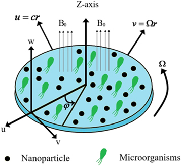
Figure 1 . Physical layout of flow problem.
Download figure:
Standard image High-resolution imageBy binomial expansion, it is possible to write as:


First-order Rivlin Erickson tensor is described by

with similarity transformations [48]:

By applying above similarity transformations, we have yield


Note that  indicates for Reynolds number,
  for material parameter,
  for Hartmann number (Magnetic parameter),
  for Prandt number,
  for Lewis number,
  for chemical reaction parameter,
  for heat source parameter,
  for Brownian number,
  for thermophoresis number,
  for bio-convective Lewis parameter,
  for Peclet parameter,
  for bio-convective Rayleigh parameter,
  for buoyancy ratio number,
  for mixed convective number,
  for Biot number,
  for solutal Biot number,
  for motile density stratification Biot number,
  for thermal relaxation parameter and
  for concentration relaxation parameter.
The surface drags, the local Nusselt number and the local Sherwood number can be described as:


Shear stresses are given by


Equation (23) substituting in equation (20), we get


where  represents local Reynolds number.
3. Numerical approach
In this section, reduced ordinary differential equations (ODEs) systems (13)–(17) with appropriate boundary conditions (18) are addressed with the Lobatto-IIIa method and a prominent bvp4c scheme via MATLAB is employed for the graphical and numerical outcomes. First, insert higher-order ODEs in the first order by adding some new variables. Let


with

4. Results and discussion
This part comprises explanation of important quantities. Numerical results have been found for the flow fields for diverse variations of appropriate numbers. Figure 2 displays nature of bio-convection Rayleigh parameter  and mixed convective number
  against axial-velocity
  The outcome discloses that axial-velocity decays for growing bioconvective Rayleigh parameter while it shows conflicting behavior for higher mixed convection parameter. To examine the impacts of Reynolds number and magnetic parameter on velocity, figure 3 is displayed. From the curves, it is detected that by increasing magnitude of both parameters i.e., Reynolds-number and the magnetic parameter, the axial-velocity diminishes. Meanwhile magnetic parameter is directly proportional to resistant force acknowledged as Lorentz force which resist the fluid motion. Figure 4 is delineated to display effects of
  and
and  for the axial velocity. The axial velocity
  falls for growing buoyancy-ratio number and dimensionless constant. To comprehend the nature of the radial velocity concentration
  for
for  and
and  we deliberately contrived some of the outlines in figure 5. It is observed that the variation in both magnetic parameter and Reynolds number, the radial velocity decreases. Figure 6 reveals the consequences of
  and
and  on velocity
  The higher valuation of both parameters dimensionless constant and buoyancy ratio parameter reduces the radial velocity profile. Figure 7 illustrates the behavior of
  and
and  for radial velocity
  The result reveals that increasing evaluation of bioconvection Rayleigh parameter diminishes the radial velocity while higher mixed convection parameter boosted the radial velocity. To understand the behavior of
  impacts of
  and
and  are portrayed in figure 8. It is perceived that for improved magnitude in magnetic number and Reynolds parameter, the velocity declines. Consequences on azimuthal velocity
  for bioconvection Rayleigh parameter
  and mixed convection parameter
  are illustrated in figure 9. It is noted that higher mixed convection parameter enhances the radial velocity while mounting values of bioconvection Rayleigh parameter moderates the radial velocity. Figure 10 precisely explains influence of
  and
and  on temperature
  The temperature amended for lager values of temperature ratio parameter and shows opposite nature for intensifying valuation of Prandtl number. The fact is that growing Prandtl number improves heat transport rate that cools system therefore temperature within boundary layer decays. In figure 11 the impacts of thermal Biot number
  and thermophoresis parameter
  for temperature profile
  are reflected. The higher valuation of Biot number and thermophoresis parameter boosted the temperature profile. Figure 12 is sketched to expose the effects of
  and mixed convection number on the temperature
  For greater values of thermal relaxation parameter
  and mixed convection parameter, the temperature profile decays. The salient features of Lewis
  and Prandtl
  parameters versus volumetric concentration are plotted in figure 13. The concentration profile of nanoparticles condenses for elevated values of both parameters. Figure 14 is captured to spot the impacts of Brownian motion parameter
  and concentration relaxation parameter
  on the volumetric concentration field
  The curves reflect that the volumetric concentration field putrefying nature for exhilarating valuation. The cause behind the decline in concentration is relation of Brownian diffusivity with Brownian diffusivity coefficient which is accountable for reducing concentration. The variation of thermophoresis parameter
  and solutal Biot number
  for concentration of nanoparticles is delineated in figure 15. Concentration field is boosted for increasing estimations of thermophoresis number and solutal Biot parameter. Figure 16 portrays the influence of activation energy
  and Reynolds number
  on concentration
  It is perceived that the concentration profile enhances for increasing variation of activation energy while conflicting behavior is watched for Reynolds number. Figure 17 is determined the nature of bio-convective Lewis
  and Peclet
  numbers for motile microorganism
  Concentration of motile micro-organism falls for amplifying values of both parameters. Such a tendency is related owing to fact that Pe conquered converse relationship with micro-organism diffusion in which motile microorganism's concentration declines. The consequences of microorganism stratified Biot number
  and bio-convective Rayleigh number
  for micro-organism field
  are deliberated in figure 18. The rising values of stratified Biot parameter and bio-convective Rayleigh number declined the microorganism's concentration. The numerical outcomes of local skin friction coefficients, Nusselt, Sherwood and microorganism density numbers are illustrated through tables 1–5. Skin frictions are upgraded for growing magnitude of magnetic number while reverse situation is watched for Sherwood, Nusselt and motile microorganism density numbers.

Figure 2. Dependence of  against
Download figure:
Standard image High-resolution image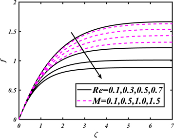
Figure 3. Dependence of  against
Download figure:
Standard image High-resolution image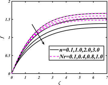
Figure 4. Dependence of  against
Download figure:
Standard image High-resolution image
Figure 5. Dependence of  against
Download figure:
Standard image High-resolution image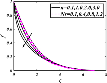
Figure 6. Dependence of  against
Download figure:
Standard image High-resolution image
Figure 7. Dependence of  against
Download figure:
Standard image High-resolution image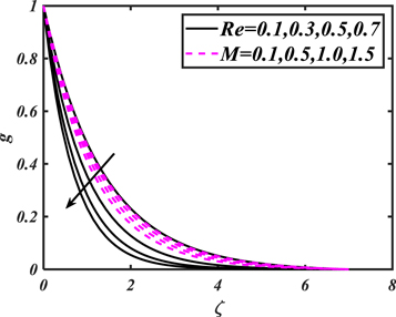
Figure 8. Dependence of  against
Download figure:
Standard image High-resolution image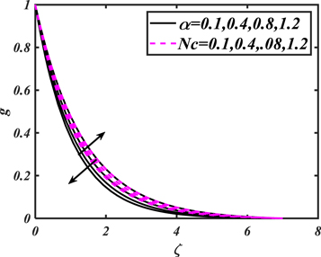
Figure 9. Dependence of  against
Download figure:
Standard image High-resolution image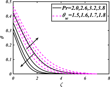
Figure 10. Dependence of  against
Download figure:
Standard image High-resolution image
Figure 11. Dependence of  against
Download figure:
Standard image High-resolution image
Figure 12. Dependence of  against
Download figure:
Standard image High-resolution image
Figure 13. Dependence of  against
Download figure:
Standard image High-resolution image
Figure 14. Dependence of  against
Download figure:
Standard image High-resolution image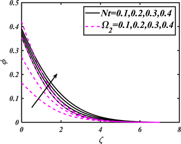
Figure 15. Dependence of  against
Download figure:
Standard image High-resolution image
Figure 16. Dependence of  against
Download figure:
Standard image High-resolution image
Figure 17. Dependence of  against
Download figure:
Standard image High-resolution image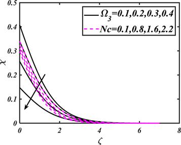
Figure 18. Dependence of  against
Download figure:
Standard image High-resolution image
Table 1. Numerical outcomes of  for variation of diverse numbers.

|

|

|

|

|

|

|
|---|---|---|---|---|---|---|
| 0.2 | 0.5 | 0.1 | 0.1 | 0.2 | 0.1 | 0.4889 |
| 0.8 | 0.6040 | |||||
| 1.2 | 0.6729 | |||||
| 0.1 | 0.1 | 0.1 | 0.1 | 0.2 | 0.1 | 0.4729 |
| 0.4 | 0.4694 | |||||
| 0.8 | 0.4640 | |||||
| 0.1 | 0.5 | 0.2 | 0.1 | 0.2 | 0.1 | 0.4874 |
| 0.8 | 0.5034 | |||||
| 1.4 | 0.5197 | |||||
| 0.1 | 0.5 | 0.1 | 0.2 | 0.2 | 0.1 | 0.4866 |
| 0.8 | 0.4982 | |||||
| 1.4 | 0.5098 | |||||
| 0.1 | 0.5 | 0.1 | 0.1 | 0.3 | 0.1 | 0.5948 |
| 0.4 | 0.6888 | |||||
| 0.5 | 0.7718 | |||||
| 0.1 | 0.5 | 0.1 | 0.1 | 0.2 | 0.2 | 0.4678 |
| 0.4 | 0.4319 | |||||
| 0.8 | 0.5288 |
Table 2. Numerical outcomes of  for variation of diverse numbers.

|

|

|

|

|
|---|---|---|---|---|
| 0.2 | 0.5 | 0.2 | 0.1 | 0.7578 |
| 0.8 | 0.8424 | |||
| 1.2 | 0.8957 | |||
| 0.1 | 0.1 | 0.2 | 0.1 | 0.7424 |
| 0.4 | 0.7430 | |||
| 0.8 | 0.7439 | |||
| 0.1 | 0.5 | 0.3 | 0.1 | 0.9059 |
| 0.4 | 1.0458 | |||
| 0.5 | 1.1691 | |||
| 0.1 | 0.5 | 0.2 | 0.2 | 0.7418 |
| 0.4 | 0.7449 | |||
| 0.8 | 0.7670 |
Table 3. Numerical outcomes of  for variation of diverse numbers.

|

|

|

|

|

|

|

|

|

|
|---|---|---|---|---|---|---|---|---|---|
| 0.2 | 0.5 | 0.1 | 0.1 | 0.2 | 0.1 | 1.0 | 0.5 | 0.2 | 0.1730 |
| 0.8 | 0.1712 | ||||||||
| 1.2 | 0.1700 | ||||||||
| 0.1 | 0.1 | 0.1 | 0.1 | 0.2 | 0.1 | 1.0 | 0.5 | 0.2 | 0.1824 |
| 0.4 | 0.1757 | ||||||||
| 0.8 | 0.1658 | ||||||||
| 0.1 | 0.5 | 0.2 | 0.1 | 0.2 | 0.1 | 1.0 | 0.5 | 0.2 | 0.2045 |
| 0.8 | 0.2044 | ||||||||
| 1.4 | 0.2042 | ||||||||
| 0.1 | 0.5 | 0.1 | 0.2 | 0.2 | 0.1 | 1.0 | 0.5 | 0.2 | 0.2046 |
| 0.8 | 0.2044 | ||||||||
| 1.4 | 0.2043 | ||||||||
| 0.1 | 0.5 | 0.1 | 0.1 | 0.3 | 0.1 | 1.0 | 0.5 | 0.2 | 0.2030 |
| 0.4 | 0.2016 | ||||||||
| 0.5 | 0.2003 | ||||||||
| 0.1 | 0.5 | 0.1 | 0.1 | 0.2 | 0.2 | 1.0 | 0.5 | 0.2 | 0.2047 |
| 0.4 | 0.2051 | ||||||||
| 0.8 | 0.2056 | ||||||||
| 0.1 | 0.5 | 0.1 | 0.1 | 0.2 | 0.1 | 2.0 | 0.5 | 0.2 | 0.2021 |
| 3.0 | 0.2155 | ||||||||
| 4.0 | 0.2234 | ||||||||
| 0.1 | 0.5 | 0.1 | 0.1 | 0.2 | 0.1 | 1.0 | 0.4 | 0.2 | 0.2058 |
| 0.8 | 0.2007 | ||||||||
| 1.4 | 0.1953 | ||||||||
| 0.1 | 0.5 | 0.1 | 0.1 | 0.2 | 0.1 | 1.0 | 0.5 | 0.4 | 0.2017 |
| 0.8 | 0.1958 | ||||||||
| 1.4 | 0.1895 |
Table 4. Numerical outcomes of  for variation of diverse numbers.

|

|

|

|

|

|

|

|

|

|

|
|---|---|---|---|---|---|---|---|---|---|---|
| 0.2 | 0.5 | 0.1 | 0.1 | 0.2 | 0.1 | 1.0 | 0.5 | 0.2 | 2.0 | 0.1975 |
| 0.8 | 0.1950 | |||||||||
| 1.2 | 0.1934 | |||||||||
| 0.1 | 0.1 | 0.1 | 0.1 | 0.2 | 0.1 | 1.0 | 0.5 | 0.2 | 2.0 | 0.1930 |
| 0.4 | 0.1934 | |||||||||
| 0.8 | 0.1939 | |||||||||
| 0.1 | 0.5 | 0.2 | 0.1 | 0.2 | 0.1 | 1.0 | 0.5 | 0.2 | 2.0 | 0.2131 |
| 0.8 | 0.2129 | |||||||||
| 1.4 | 0.2127 | |||||||||
| 0.1 | 0.5 | 0.1 | 0.2 | 0.2 | 0.1 | 1.0 | 0.5 | 0.2 | 2.0 | 0.2131 |
| 0.8 | 0.2130 | |||||||||
| 1.4 | 0.2129 | |||||||||
| 0.1 | 0.5 | 0.1 | 0.1 | 0.3 | 0.1 | 1.0 | 0.5 | 0.2 | 2.0 | 0.2268 |
| 0.4 | 0.2353 | |||||||||
| 0.5 | 0.2413 | |||||||||
| 0.1 | 0.5 | 0.1 | 0.1 | 0.2 | 0.2 | 1.0 | 0.5 | 0.2 | 2.0 | 0.2133 |
| 0.4 | 0.2137 | |||||||||
| 0.8 | 0.2035 | |||||||||
| 0.1 | 0.5 | 0.1 | 0.1 | 0.2 | 0.1 | 2.0 | 0.5 | 0.2 | 2.0 | 0.2203 |
| 3.0 | 0.2334 | |||||||||
| 4.0 | 0.2415 | |||||||||
| 0.1 | 0.5 | 0.1 | 0.1 | 0.2 | 0.1 | 1.0 | 0.4 | 0.2 | 2.0 | 0.2103 |
| 0.8 | 0.2174 | |||||||||
| 1.4 | 0.2198 | |||||||||
| 0.1 | 0.5 | 0.1 | 0.1 | 0.2 | 0.1 | 1.0 | 0.5 | 0.4 | 2.0 | 0.2037 |
| 0.8 | 0.1874 | |||||||||
| 1.4 | 0.1744 | |||||||||
| 0.1 | 0.5 | 0.1 | 0.1 | 0.2 | 0.1 | 1.0 | 0.5 | 0.2 | 3.0 | 0.2285 |
| 4.0 | 0.2378 | |||||||||
| 5.0 | 0.2442 |
Table 5. Numerical outcomes of  for variation of diverse numbers.

|

|

|

|

|

|

|

|

|
|---|---|---|---|---|---|---|---|---|
| 0.2 | 0.5 | 0.1 | 0.1 | 0.2 | 0.1 | 0.1 | 0.8 | 0.1975 |
| 0.8 | 0.1950 | |||||||
| 1.2 | 0.1934 | |||||||
| 0.1 | 0.1 | 0.1 | 0.1 | 0.2 | 0.1 | 0.1 | 0.8 | 0.1978 |
| 0.4 | 0.1979 | |||||||
| 0.8 | 0.1980 | |||||||
| 0.1 | 0.5 | 0.2 | 0.1 | 0.2 | 0.1 | 0.1 | 0.8 | 0.1972 |
| 0.8 | 0.1969 | |||||||
| 1.4 | 0.1966 | |||||||
| 0.1 | 0.5 | 0.1 | 0.2 | 0.2 | 0.1 | 0.1 | 0.8 | 0.1972 |
| 0.8 | 0.1970 | |||||||
| 1.4 | 0.1968 | |||||||
| 0.1 | 0.5 | 0.1 | 0.1 | 0.3 | 0.1 | 0.1 | 0.8 | 0.1989 |
| 0.4 | 0.1963 | |||||||
| 0.5 | 0.1940 | |||||||
| 0.1 | 0.5 | 0.1 | 0.1 | 0.2 | 0.2 | 0.1 | 0.8 | 0.2019 |
| 0.4 | 0.2024 | |||||||
| 0.8 | 0.2035 | |||||||
| 0.1 | 0.5 | 0.1 | 0.1 | 0.2 | 0.1 | 0.2 | 0.8 | 0.2038 |
| 0.4 | 0.2079 | |||||||
| 0.8 | 0.2154 | |||||||
| 0.1 | 0.5 | 0.1 | 0.1 | 0.2 | 0.1 | 0.1 | 1.0 | 0.2101 |
| 2.0 | 0.2326 | |||||||
| 3.0 | 0.2434 |
5. Conclusions
This article comprises the computational analysis of Sutterby nanoliquid flow over a disk with the effects of activation energy, magnetic field and motile microorganisms' concentration. Built-in bvp4c technique is used to solve the PDEs to ODEs via appropriate similarity transformations. The velocities and volumetric concentration of nanoparticles is falls for growing values of Reynolds number. Both temperature ratio and thermophoresis parameters raised the temperature and the concentration. The volumetric concentration of nanomaterial rises for thermophoresis number while shows opposite nature for Prandtl and Lewis parameters. The boosting values of bioconvection Lewis number, Peclet number and bioconvection Rayleigh number decay the motile microorganisms' concentration.
Acknowledgments
This project was funded by the Deanship of Scientific Research (DSR) at King Abdulaziz University, Jeddah, under grant no. G: 643-247-1441. The authors, therefore, acknowledge with thanks DSR for technical and financial support.
Data availability statement
All data that support the findings of this study are included within the article (and any supplementary files).