


Abstract
We study the stability and characteristics of two-dimensional (2D) quasi-isotropic quantum droplets (QDs) of fundamental and vortex types, formed by binary Bose–Einstein condensate with magnetic quadrupole–quadrupole interactions (MQQIs). The magnetic quadrupoles are built as pairs of dipoles and antidipoles polarized along the x-axis. The MQQIs are induced by applying an external magnetic field that varies along the x-axis. The system is modeled by the Gross–Pitaevskii equations including the MQQIs and Lee-Huang-Yang correction to the mean-field approximation. Stable 2D fundamental QDs and quasi-isotropic vortex QDs with topological charges  are produced by means of the imaginary-time-integration method for configurations with the quadrupoles polarized parallel to the system's two-dimensional plane. Effects of the norm and MQQI strength on the QDs are studied in detail. Some results, including an accurate prediction of the effective area, chemical potential, and peak density of QDs, are obtained in an analytical form by means of the Thomas-Fermi approximation. Collisions between moving QDs are studied by means of systematic simulations.
Export citation and abstract BibTeX RIS

Original content from this work may be used under the terms of the Creative Commons Attribution 4.0 license. Any further distribution of this work must maintain attribution to the author(s) and the title of the work, journal citation and DOI.
1. Introduction
In 2015, Petrov had proposed a scheme for suppression of the collapse in the binary (two-species) Bose–Einstein condensate (BEC) in the three-dimensional (3D) space with  , where g12 is the strength of the inter-species attraction, while g11 and g22 are strengths of the intra-species self-repulsion [1]. The stabilization of the system against the collapse is provided by the Lee-Huang-Yang (LHY) effect, i.e. corrections to the mean-field BEC dynamics induced by quantum fluctuations [2]. The analysis had predicted the arrest of the collapse and formation of stable quantum droplets (QDs) filled by the ultra-diluted quantum fluid. Following the prediction, QDs have been created in a mixture of two hyperfine atomic states of 39K, with the quasi-2D [3, 4] and fully 3D [5] shapes, as well as in a heteronuclear mixture of 23Na and 87Rb [6] atoms. The use of the LHY effect has also made it possible to create QDs in single-component dipolar bosonic gases of dysprosium [7] and erbium [8] atoms. The further analysis has demonstrates that the LHY corrections take different forms in 1D, 2D, and 3D configurations [9].
Studies of QDs have drawn much interest in very different contexts [10–57] . Various phenomena, such as the spin–orbit coupling [58], supersolidity [59, 60], and metastability [61] can be emulated in BECs under the action of the LHY corrections. Further, stable semi-discrete vortex QDs were predicted in arrays of coupled 1D cigar-shaped traps [62], and the symmetry breaking of QDs has been studied in a dual-core trap [63].
In particular, an interesting possibility is to create stable solitary vortices, i.e. QDs with embedded vorticity (traditional quantized vortices in BEC are eddy states supported by a flat background, i.e. they are 2D dark solitons [64], while solitary vortices resemble bright matter-wave solitons). Such modes are often subject to the azimuthal modulational instability that develops faster than the collapse, splitting the vortices into fragments. Therefore, stability conditions for vortex QDs become increasingly stricter with the increase of their winding number (alias the topological charge). The possibility for the stabilization of the vortex modes has been revealed by studies of BEC systems under the action of spatially periodic and quasiperiodic lattice potentials [65–77]. Recently, stable QDs in 2D square lattices [78] and ring-shaped QDs with explicit and hidden vorticity in a radially periodic potential [79, 80] have been predicted ('hidden vorticity' means as a vortex-antivortex bound state in a two-component system with zero total angular momentum [74]). In the free space, stable 2D matter-wave solitons were predicted in microwave-coupled binary condensates [81], and solutions for stable semi-vortices, i.e. 2D [82] and 3D [83] spin–orbit-coupled two-component matter-wave solitons carrying vorticity in one component, are known too.
In dipolar BECs, QDs have been observed in the form of 3D self-bound states. In the 2D geometry, the coherence of QDs was explored in [84]. In [85], the ground-state properties and intrinsic excitations of QDs in dipolar BECs were studied in detail. The previous studies demonstrate that QDs in dipolar BECs feature strong anisotropy of their density profile in the free space, but they do not carry vorticity. In [86], isotropic vortex QDs with the dipoles polarized parallel to the vortical pivot were constructed and found to be completely unstable. Thus, creating stable vortex QDs in BECs with dipole–dipole interactions (DDI) remains a fundamental problem. Recently, solutions for 2D fundamental QDs in dipolar BEC with the dipoles oriented perpendicular to the system's plane have been produced [87]. Furthermore, Li et al have proved that dipolar BEC offers a unique possibility to predict stable 2D anisotropic vortex QDs with the vortex axis oriented perpendicular to the polarization of dipoles [88]. Hence, modifying the attractive nonlinearity by introducing DDI is a promising direction for the stabilization of vortex QDs in BEC. The objective of the present work is to demonstrate that the stabilization is also possible with the help of long-range quadrupole-quadrupole interactions (QQI) between particles in BEC. Previously, the formation of solitons in QQI-coupled BEC was addressed in models that did not include the LHY terms [89–93], which made it more difficult to stabilize the self-trapped states in the BEC.
Electric quadrupoles may be built as tightly bound pairs of dipole and antidipoles directed perpendicular to the system's (x, y) plane, i.e. along the z-axis. By applying an external gradient electric field along the z-axis the electric QQI (alias EQQI) can be induced. The potential of the interaction between two electric quadrupoles in this configuration is written in the polar coordinates  as
as

where Q is the quadrupole moment, r is the distance between the quadrupoles, and θ is the angle between the vector connecting the quadrupoles and the line connecting the dipole and antidipole inside the quadrupole. Averaging potentials (1) over the angular range  yields the respective mean values:

According to equation (2), the EQQI represent the attractive interaction.
Relatively large electric quadrupole moments are featured by some small molecules [94] and by bound states in the form of alkali diatoms [95]. These particles can be used to create BEC in which EQQI plays an essential role. In [89], the creation of quadrupolar matter-wave solitons in the 2D free space was predicted, with a conclusion that, in the presence of EQQI, the solitons feature a higher mass and stronger anisotropy than their DDI-maintained counterparts, for the same environmental parameters. Possibilities of building 2D (quasi-) discrete matter-wave solitons composed of quadrupole particles trapped in deep isotropic and anisotropic optical-lattice potentials was demonstrated in [90, 91], respectively. In [96], soliton solutions of the mixed-mode and semi-vortex types were constructed in binary quadrupolar BECs including spin–orbit coupling.
Magnetic quadrupoles can be built as tightly bound dipole-antidipole pairs directed along a particular axis (x). They can be polarized parallel to each other by a gradient magnetic field also directed along the x-axis. The potential of the magnetic quadrupole–quadrupole interactions (MQQI) is

cf equation (1). Unlike EQQI, which is attractive on the average, for MQQI the mean value of potential (3) corresponds to repulsion:

cf equation (2).
In the usual mean-field approximation, which is represented by the Gross–Pitaevskii (GP) equation for the single-particle wave function ψ [97], BEC cannot maintain localized states with the help of MQQI, unless an external trapping potential is used [98]. However, the above-mentioned proposal to create QDs in BEC by means of the LHY correction to the mean-field approximation [1, 9] suggests a possibility to predict self-trapped objects supported by the QQI. Note that the LHY terms take different forms for different spatial dimensions. In 3D, this term in the corrected GP equation is proportional to  , with the sign representing self-repulsion [1]. In 2D, the combined mean-field-LHY term is

where  is a positive coefficient, and n0 is the reference density [9] (its typical value is
  cm−3). Expression (5) implies the attraction at
  , and repulsion at
  . Finally, in 1D, the LHY term is proportional to
  , with the sing corresponding to the self-attraction, which helps to build solitons and QDs in the effectively one-dimensional condensate [9].
In this work, we produce 2D solutions for self-bound states, including ones with embedded vorticity, in magnetic quadrupolar BEC, taking the corresponding LHY correction into account. Following the original proposal [1, 9] which derived the correction for the two-component BEC, we also address the two-component system. In this connection, it is relevant to stress that the LHY correction to the GP equation for the dipolar BEC has the same form (in particular, being  in 3D) as in the case of the BEC with contact-only atomic interactions [99, 100]. Accordingly, the same is true for the BEC featuring the long-range MQQI in the combination with the local nonlinearity.
We here consider the 2D model with coordinates  , including a gradient magnetic field oriented along the x direction. This field is induced by a tapered solenoid, as shown schematically in figure 1. In this configuration, the MQQI, defined as per equation (3), represents self-repulsion, while the local interaction, combining the mean-field and LHY terms according to equation (5) may account for attraction. The self-trapping of QDs is achieved through competition between these terms.

Figure 1. The system's scheme. Quadrupoles are built as tightly-bound dipole-antidipole pairs, polarized along the x axis by means of the gradient magnetic field (with the local strength being a linear function of x), see [90]. This field can be imposed by the tapered solenoid, as shown in the figure. The expression of the magnetic field at any point xp
belonging to the x-axis of the tapered solenoid is produced by the integration of ![$\mathrm{d}B_{x}\sim \mu _{0}nI[r_{2}-(r_{2}-r_{1})x/h]\mathrm{d}x/[(r_{2}-(r_{2}-r_{1})x/h)^{2}+(x-x_{p})^{2}]^{3/2}\mathrm{d}x $](https://content.cld.iop.org/journals/1367-2630/26/5/053037/revision2/njpad49c4ieqn13.gif) , where r1 and r2 are radii of the upper and lower bottom surfaces of the solenoid, h is the length of the solenoid, I is the current, and n is the number of turns of the coil. Red and green rectanges represent two components of the bosonic mixture.
, where r1 and r2 are radii of the upper and lower bottom surfaces of the solenoid, h is the length of the solenoid, I is the current, and n is the number of turns of the coil. Red and green rectanges represent two components of the bosonic mixture.
Download figure:
Standard image High-resolution imageFundamental QDs and quasi-isotropic vortical ones are produced by the analysis presented below. Effects of the norm and strength of the MQQI are systematically studied. The rest of the paper is structured as follows. The model is introduced in section 2. Numerical findings and some analytical estimates are summarized in section 3. The dynamics of the QDs are the focus of section 4. The paper is concluded in section 5.
2. The model
We aim to consider two-component QDs in the magnetic quadrupolar BEC, which is made effectively two-dimensional by the application of strong confinement in the transverse direction, with confinement size  m. The orientation of individual quadrupoles is fixed as in figure 1. The system's dynamics are governed by the 2D coupled GP equations, produced by the reduction of the full 3D GP system. The 2D equations include the LHY terms, as derived in [9]. In the scaled form, they are written as [88, 99, 100]


where  are wave functions of the two components, with density
  normalized to the above-mentioned reference density n0 (cf equation (5)), r = {x,y} is the set of coordinates measured in units of
  (i.e. essentially, measured in microns),
  , the unit of time t is
  ms, assuming that the mass of the particles is
  proton masses, while
  and
and  , which are proportional to the respective scattering lengths of the inter-particle collisions, are strengths of the contact intra-component repulsion and inter-component attraction, respectively. Further, coefficients γ and
  (see [90]) represent the LHY correction [9] and MQQI, respectively. The MQQI kernel is

cf equation (3), where  and
and  is the cutoff, which is determined by the above-mentioned transverse confinement size, that is set to be 1, as said above.
Following [9], we focus the consideration on the symmetric system, with  and
and  , thus reducing equations (6) and (7) to a single equation in the finally scaled form:

where κ remains the single control parameter, while b = 1 is fixed in equation (8), in accordance with what is said above. Dynamical invariants of equation (9) is the total norm,

which is proportional to the number of atoms in the BEC, and the total energy, that includes the mean-field and LHY terms:

Moving states also conserve the integral momentum,  , where
  stands for the complex conjugate. Strictly speaking, the anisotropy present in equations (8) and (9) breaks the conservation of the angular momentum in the present setting. In fact, the QDs in our system are found to be quasi-isotropic (as shown below), therefore the angular momentum is approximately conserved.
The units of coordinates and time in equation (9) are tantamount, as said above, to  m and 1 ms, respectively, while undoing the rescaling demonstrates that the value of the scaled norm N = 100 corresponds to
  particles in the underlying BEC.
We look for stationary solutions to equation (9), which represents stationary QDs with the chemical potential µ in the usual form,

where  is a wave function which is real for fundamental states, and complex for vortical ones. Stationary QD solutions were produced by means of the well-known imaginary-time-propagation (ITP) method [101–103] applied to equation (9).
3. Stationary solutions for the quantum droplets (QDs)
The strength of the MQQI, κ, and the total norm, N, are used as control parameters in the present analysis. To generate stationary states, the ITP method was initiated with the initial guess

where α and A are real constants, r and θ are 2D polar coordinates, and integer S is vorticity (topological charge, alias winding number, S = 0 corresponding to the ground state). Further, stability of the stationary QD states was verified by direct simulations of the perturbed real-time evolution. The simulations were run by dint of the split-step Fourier-transform algorithm, adding random noise at the 1% amplitude level to the input, taking the input as ![$\psi = [1+\varepsilon ^{^{^{\prime} }}f(x,y)]\cdot \phi ^{\left( S\right) }\left( x,y\right) $](https://content.cld.iop.org/journals/1367-2630/26/5/053037/revision2/njpad49c4ieqn33.gif) , where
, where  and
and  is a random function with the value range
 ![$[0,1]$](https://content.cld.iop.org/journals/1367-2630/26/5/053037/revision2/njpad49c4ieqn36.gif) , which can be generated by the standard 'rand' routine.
, which can be generated by the standard 'rand' routine.
3.1. Fundamental QDs
Typical examples of numerically constructed stable quasi-isotropic fundamental QDs with S = 0 are displayed in figure 2. The parameters are  in (a) and (1000, 0.5) in (b). The stability of these QDs was confirmed by direct simulations of their perturbed evolution, as shown in figures 2(c) and (d). Similar to QDs in binary bosonic gases with contact-only interactions, the quasi-isotropic QDs in the quadrupolar BEC generally feature flat-top density profiles. In this case, one can apply the Thomas-Fermi (TF) approximation, neglecting the gradient term in energy (11). The corresponding approximation yields

where  ,
,  is the effective area of the flat-top QD, and

with  taken as per equation (8), is an effective measure of the repulsive nonlocality. Then, one can obtain the equilibrium density ne
and the effective area AS
of the quasi-isotropic QD from the energy-minimum condition
taken as per equation (8), is an effective measure of the repulsive nonlocality. Then, one can obtain the equilibrium density ne
and the effective area AS
of the quasi-isotropic QD from the energy-minimum condition  , which yields


The chemical potential corresponding to the equilibrium density (17) is

Figure 2. Typical examples of stable quasi-isotropic fundamental quantum droplets (QDs) produced by input ( 13) with S = 0. Panels (a) and (b) display the density profiles of the QDs with  and (1000, 0.5). (c) and (d): The perturbed evolution of the QDs from (a) and (b), produced by simulations of equation ( 9) with the 1% random noise added to the input.
Download figure:
Standard image High-resolution image

Further, as a characteristics of the QDs, we define their effective area:

Comparing the results for κ = 0.1 and κ = 0.5 in figure 2 , we conclude that the effective area is larger in the latter case, as is also seen in figure 3(a1).

Figure 3. The first column (a1)–(a3): the effective area (Aeff), peak density (Ip
), and chemical potential ( ) of the fundamental quasi-isotropic QDs as functions of the strength of
  with the norm N = 500. The second column (b1)–(b3): the dependence of Aeff, Ip
and
with the norm N = 500. The second column (b1)–(b3): the dependence of Aeff, Ip
and  on the norm, N, with
  . Here, the solid blue line shows results of the numerical simulations, and the dotted red line shows the analytical approximation, see equations (16)–(18), for Aeff, Ip
and
. Here, the solid blue line shows results of the numerical simulations, and the dotted red line shows the analytical approximation, see equations (16)–(18), for Aeff, Ip
and  , respectively.
Download figure:
Standard image High-resolution imageFor the fixed norm, the dependence of the effective area Aeff on the MQQI strength κ is shown in figure 3(a1), which indicates that the effective area exponentially grows the increase of κ. Here, the solid blue and dotted red lines show, respectively, results of the numerical simulations and the analytical results, produced by equation (16), the two curves being almost identical.
Next, we show the peak density, Ip
( ), and the chemical potential µ of the stable quasi-isotropic QDs as functions of the MQQI strength κ in figures 3(a2) and (a3), respectively. Figure 3(a2) shows that Ip
decreases with κ, which is also in agreement with equation (17), in which the peak density decays exponentially with the increase of the MQQI strength.
), and the chemical potential µ of the stable quasi-isotropic QDs as functions of the MQQI strength κ in figures 3(a2) and (a3), respectively. Figure 3(a2) shows that Ip
decreases with κ, which is also in agreement with equation (17), in which the peak density decays exponentially with the increase of the MQQI strength.
In figures 3(b1)–(b3), we fix the MQQI strength κ, to address the dependence of the effective area Aeff, peak density Ip
, and chemical potential µ on the total norm N. Similar to the 2D anisotropic QDs in dipolar BECs, the effective area of the quasi-isotropic QDs grows linearly with the increase of the total norm, see equation (16), which is a natural feature of flat-top modes. In figure 3(b2), the peak density saturates at  , if N is sufficiently large, which corroborates that the superfluid filling the QDs is incompressible, as demonstrated first in [1]. According to equation (17), the theoretical prediction for the equilibrium density is about 0.440, which is very close to the numerical results (see the red dashed line in figure 3(b2)). The
  curves in figure 3(b3) feature a negative slope, i.e.
  , satisfying the Vakhitov-Kolokolov (VK) criterion [104], which is a necessary stability condition for self-trapped modes maintained by any self-attractive nonlinearity. Figure 3(b3) shows that the chemical potential saturates at
  when the norm is large. The TF-predicted value given by equation (18) is
  (see the red dashed line in figure 3(b3)). As shown in figure 3, all the numerical results agree well with the analytical predictions provided by equations (16)–(18).
3.2. QDs with embedded vorticity
The present system maintains stable vortex QDs (VQDs) as well. A typical example of a numerically constructed one with winding number S = 1, produced by input (13) with S = 1, is displayed in figure 4, for N = 1000, and κ = 0.1. The stability of these VQDs was confirmed by direct simulations of its perturbed evolution, see figure 4(c), where 1% random noise is added to the input.

Figure 4. (a) and (b): The density and phase patterns of a stable quasi-isotropic VQD (vortex QD) produced by equation (13) with winding number S = 1 and  . (c) Simulations of the perturbed evolution of the VQDs shown in panel (a) with
  random noise added to the input.
Download figure:
Standard image High-resolution imageTo systematically study characteristics of the VQD families, we define their aspect ratio and average angular momentum as follows:


where  and
and  represent the effective lengths of the VQDs in the
  -direction, and the angular-momentum operator, respectively:


In particular,  indicates that the VQDs manifest anisotropy with the elongation along the x-direction, while
  implies their isotropy [88].
The aspect ratio Al
and average angular momentum  of stable VQDs with N = 500, defined as per equations (20)–(24), are displayed in figures 5(a1) and (a2), respectively, as functions of the MQQI strength κ, varying in interval
  Note that, according to figure 3(a1), the effective area of QDs exponentially grows with the increase of κ, making the calculations more difficult. For this reason, we here present the results for κ < 1. Figures 5(b1) and (b2) display the VQD characteristics Al
and
Note that, according to figure 3(a1), the effective area of QDs exponentially grows with the increase of κ, making the calculations more difficult. For this reason, we here present the results for κ < 1. Figures 5(b1) and (b2) display the VQD characteristics Al
and  as functions of the norm N, with κ = 0.1. In panel 5(a1), the aspect ratio attains a maximum value 1.1742 and approaches 1.0677 at
  . Figure 5(a2) depicts the respective orbital momentum, whose average value is 0.9955. In panels 5(b1) and (b2), the aspect ratio and orbital momentum have values of
  and
and  , respectively. These findings indicates that the system with the repulsive MQQI maintains stable quasi-isotropic VQDs, whose aspect ratio is slightly larger than 1. In this connection, it is relevant to mention that for the fundamental QD modes considered above, values of the aspect ratio are also approximately equal to 1, as the density distribution in those modes seem to be nearly axisymmetric (isotropic).

Figure 5. Panels (a1) and (a2) display the aspect ratio Al
and average angular momentum  of stable quasi-isotropic VQDs with N = 500, respectively, as functions of the MQQI strength
  . Panels (b1) and (b2) display the values, (Al
,
. Panels (b1) and (b2) display the values, (Al
,  ), for VQDs as functions of the norm N, with
  . The red dashed line designate the unit levels.
Download figure:
Standard image High-resolution imageSimulations of in elastic collisions between moving stable VQDs with S = 1 (see figure 10 below) demonstrate that they may merge into a single breather with angular momentum (21) close to  . This fact suggests that stable VQDs with S = 2 may exist too. A typical example of such a vortex state, produced by input equation (13) with S = 2, is displayed in figure 6, with the same parameters as in figure 4. The respective values given by equations (20) and (21) for this double VQD are
  and
and  at
at  .
.

Figure 6. Panels (a) and (b): The density and phase patterns of a stable VQD with winding number S = 2. The other parameters are the same as in figure 4. (c) Simulations of the perturbed evolution of the VQD shown in panels (a) and (b), with 1% random noise added to the input.
Download figure:
Standard image High-resolution imageThe family of VQDs with S = 2 are characterized by dependences of their chemical potential µ on κ and N, as shown in figures 7(a) and (b). Next, we fix the characteristic value of the MQQI strength, κ = 0.3, to study a relation between the chemical potential µ of VQDs with S = 2 and their norm N. Figure 7(a) shows that the  curve has a negative slope, satisfying the VK criterion. It is worthy to note that, for the current fixed values S = 2 and κ = 0.3, the VQDs are stable in a finite interval,
  , see the red line in figure 7(a), while the black dotted segments of the curves represent unstable states, for the same parameters. In figure 7(b), with N = 1000, the stable VQDs with S = 2 populate the area of κ < 0.45.

Figure 7. (a) and (b): The chemical potential of the stable VQDs with S = 2 versus N (at  ) and
) and  (at N = 1000), respectively. The red solid and black dotted segments of the curves represent, respectively, stable and unstable states.
Download figure:
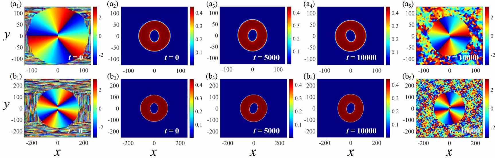
Standard image High-resolution imageWe have also constructed VQD states with higher vorticities,  , as shown in figure 8. Typical examples of QDs with S = 3 and S = 4, with parameters
  and
and  , are displayed in figures 8(a1)–(a5) and (b1)–(b5), respectively. Figures 8(a1),(b1) and (a5),(b5), respectively, display the initial (t = 0) and final (
 ) phase patterns of for S = 3 and 4. Figures 8(a2)–(a4) and (b2)–(b4) show the density patterns at t = 0, 5000, and
  . The simulations demonstrate that those QDs are stable and feature quasi-isotropic shapes. According to equation (20), we have found
  in figure 8(a4) and
  in figure 8(b4). Further, according to equation (21), we have calculated the average angular momentum of these QDs at
  ,
,  in figure 8(a4) and
  in figure 8(b4), which exhibit a small deviation from the corresponding initial values of the angular momentum.

Figure 8. Typical examples of quasi-isotropic VQDs with  and
and  . (a1),(b1) and (a5),(b5) Display the VQD phase patterns at t = 0 and
  , respectively. Panels (a2)–(a4) and (b2)–(b4) show the density patterns of the VQDs at t = 0, 5000, and
  , respectively.
Download figure:
Standard image High-resolution image4. Dynamics of the quantum droplets (QDs)
It is well known that stable QDs in binary BECs can be set in motion by opposite kicks with magnitude ±η applied along the x- or y -direction, which suggests to consider collisions between two QDs moving in the opposite directions [105, 106]. The kicks can be readily applied by optical pulses shone through the tapered solenoid.
Here, we address the collisions between the QDs moving in the x direction. The corresponding initial states are constructed as

where  represents the stationary quasi-isotropic QDs initially centered at
  . It is necessary to choose x0 large enough so that the two QDs are initially placed far from each other, avoiding any overlap.
4.1. Collisions between fundamental QDs
First, we consider the collisions between moving fundamental QDs (S = 0). In [63], where collisions between two-component QDs have been considered in the model with contact interactions, the simulations demonstrated a trend to inelastic outcomes produced by the collisions between QDs in the in-phase configuration. In [42], the collisional dynamics has been studied for two symmetric QDs with equal intra-species scattering lengths and equal densities of both components. In [88], the collisions between moving 2D anisotropic vortex QDs have been studied, demonstrating the formation of bound states with a vortex-antivortex-vortex structure.
We have produced typical results for the collisions generated by input (25) with ( ) = (
) = ( ). The results are shown in figure 9. Figures 9(a1)–(a6) show the result of the strongly inelastic collision between moving QDs set in motion by kicks ±0.1. The result is fusion of the two fundamental QDs into a quadrupole breather. It stretches periodically in the x and y directions, resembling the dynamics featured by a liquid drop [42]. When the initial kicks increase to ±0.12, quasi-elastic outcomes of the collision are observed. In this case, figures 9(b1)–(b6) show that the colliding droplets separate into another pair of droplets, slowly moving in the perpendicular direction, i.e. the collision leads to the deflection of the direction of motion by 90o. Similar results were mentioned in [42, 87] . When the norm is fixed, the outcome of the collision is mainly determined by the velocity, i.e. by kick η [42, 63, 107]. If the collision speed exceeds a critical value, an inelastic collision takes place. A typical example of an inelastic collision of two quasi-isotropic fundamental QDs is shown in figures 9(c1)–(c6). After the collision, they split into several fragments. Note that the norm and the MQQI strength (both of which affect the QD's size) also affects the outcome of the collision. We do not consider these effects in detail here.

Figure 9. Examples of collisions between moving quasi-isotropic fundamental QDs, produced by input (25) with  . Initial parameters of the QDs are
  . (a1)–(a6): A strongly inelastic collision of two QDs, set in motion by kicks ±0.1. (b1)–(b6): A collision initiated by kicks ±0.12. (c1)–(c6): An inelastic collision in the case of strong kicks, ±0.3, which implies the collision with a large relative velocity.
Download figure:
Standard image High-resolution image4.2. Collision between moving vortex quantum droplets (VQDs)
Next, we consider collisions between moving VQDs. For the input given by equation (25) with ( ) = (
) = ( ), several typical outcomes of the collision are presented in figure 10. In figures 10(a1)–(a6), the collision with a small relative speed, initiated by small kicks (here, they are ±0.01), demonstrates that the VQDs bounce back, keeping their original vorticities, as a result of the contactless collision. According to equation (21), angular momenta of the two droplets in figure 10(a6) are
  . It is worth noting that the mutual rebound does not occur in the in the case of the collision of fundamental QDs, as seen in figure 9. By gradually increasing the kicks to ±0.04, the colliding VQDs merge and eventually split into a couple of non-vortical fragments, see figures 10(b1)–(b6). The simulations demonstrate a trend to the merger of the colliding VQDs into a vortex breather. In particular, this outcome, corresponding to the initial kicks ±0.06, is observed in figures 10(c1)–(c6). The emerging breather absorbs 86.34% of the total norm in figure 10(c6). The angular momentum of the breather is
  , which is relatively close to 2. The VQDs being quasi-isotropic, the average angular momentum is approximately conserved, as mentioned above. This result suggests the existence of stable VQDs with vorticity S = 2. As demonstrated above, stable stationary VQDs withe S = 2 are indeed available.

Figure 10. Several typical examples of collisions between moving quasi-isotropic vortex quantum droplets (VQDs), by inputting expression (25) with  , which is selected with
  . (a1)–(a6) The contactless collision initiated by kick
  . (b1)–(b6) Collision with the kick
  . (c1)–(c6) Collision with the kick,
  .
.
Download figure:
Standard image High-resolution image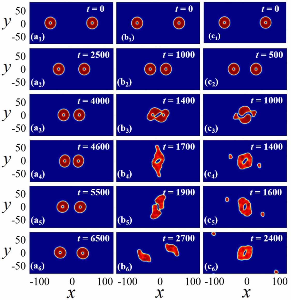
5. Conclusion
The purpose of this work is to establish the stability and characteristics of 2D quasi-isotropic QDs in magnetic quadrupolar BECs. The system is modeled by the coupled GP including the LHY terms, which represent the correction to the mean field theory produced by quantum fluctuations. Stable quasi-isotropic QDs of the fundamental and vortex types (with topological charges  ) have been produced by means of imaginary-time simulations. The effect of the norm and strength of the MQQIs, κ, on the QDs were studied in detail. It was thus found that the QD's size increases with the increase of κ. For stable QDs, the dependence between the chemical potential and total norm obeys the VK criterion. The dependence of the effective size and peak density of the QDs on κ and norm N have been studied too. The results of the numerical simulation are consistent with the analytical predictions produced by the TF approximation. Typically, the predicted stable QDs have the size in the range of
  m, with the number of particles in the range of
  , with density
  cm−3.
cm−3.
Collisions between moving QDs have been also studied systematically, for the fundamental and vortex droplets alike. For moving fundamental QDs, the strongly inelastic, quasi-elastic, and inelastic outcomes of the collision have been observed. For moving vortex QDs, a noteworthy results is the contactless rebound of the colliding droplets.
The present analysis can be extended further. In particular, it is relevant to look for essentially anisotropic QDs, especially higher-order vortical ones, in the framework of the present model. A challenging option is to seek for stable vortex QDs in the full three-dimensional setting including MQQI.
Acknowledgments
This work was supported by the Natural Science Foundation of GuangDong Province through Grant Nos. 2024A1515030131 and 2021A1515010214, GuangDong Basic and Applied Basic Research Foundation through Grant No. 2023A1515110198, National Natural Science Foundation of China through Grant Nos. 12274077 and 11905032, the Research Fund of the Guangdong-Hong Kong-Macao Joint Laboratory for Intelligent Micro-Nano Optoelectronic Technology through Grant No. 2020B1212030010, and Israel Science Foundation through Grant No. 1695/22.
Data availability statement
No new data were created or analysed in this study.