


Abstract
A general acoustic force field can be decomposed into a conservative gradient force (GF) and a non-conservative scattering force (SF), which have very different physical and mathematical properties. However, the profiles of such forces for Mie particles are unknown, let alone their underlying physics. Here, by using a fast Fourier transform approach, we calculated the GF and SF for spherical particle of various sizes and various incident waves. For the same focused incident waves, the normalized GF and SF are similar for different particle sizes, while the total force can be quite different owing to the varying relative strength between the GF and SF. GF and SF possess symmetries that are not found in the incident waves, indicating that these physically and mathematically distinct forces have symmetries that are hidden from the beam profile. For a vortex beam carrying a well-defined topological charge, acoustic forces alone cannot trap particles.
Export citation and abstract BibTeX RIS

Original content from this work may be used under the terms of the Creative Commons Attribution 4.0 license. Any further distribution of this work must maintain attribution to the author(s) and the title of the work, journal citation and DOI.
1. Introduction
Optical tweezers (OTs), a well-established, non-invasive, contactless manipulation technique, were proposed in 1986 [1]. Subsequently, the technique was applied to manipulate microscopic, or even nanoscopic objects, such as colloids and living biological particles [2–4]. Nevertheless, OTs still have some shortcomings such as the heat they generate on absorbing particles and the minute force they can exert. As an alternative, acoustic tweezers (ATs) can also serve as versatile, non-invasive tools for trapping and manipulating particles [5–15]. And ATs have been implemented using various techniques. For instance, they have been achieved through the utilization of single beam [9], hologram [12], ultrasonic attenuation [16], beating sound waves [17], and other methods [10]. Due to the orders of magnitude slower wave speed, a sound wave is generally able to exert much larger forces than its optical counterpart at the same intensity. Also, a particle that absorbs light may not absorb acoustic waves, thus allowing ATs to serve as a complementary tool of OTs. While both techniques are operable for microparticles, nanoparticles are better trapped by OTs, whereas ATs are better suited for millimeter-sized particles [10, 18, 19]. Moreover, acoustic waves typically have better biocompatibility since it is more transparent to living issues than optical waves [19, 20].
The acoustic radiation force arises from momentum transfer during the scattering of sound waves. The system consisting of a particle immersed in an acoustic field is non-conservative and non-Hermitian since sound waves can also exchange energy with the particle owing to its open nature [21, 22]. A general force field  , according to the Helmholtz's theorem, can always be decomposed into a curl-less conservative force field
  fulfilling
  , and a divergence-less non-conservative force field
  fulfilling
  , where
  and
and  are scalar and vector potential fields, respectively. We call
  the gradient force (GF) and
  the scattering force (SF). GF and SF have very different mathematical and physical properties and applications. GF is a conservative force that is responsible for particle trapping, while SF is a non-conservative force that can transport or revolve particles. Note that SF cannot trap particles by just itself as stated by Earnshaw's theorem [23]. However, writing down the analytical expression of GF and SF for an arbitrary particle is quite difficult. It is possible for Rayleigh particles [24, 25], but not for larger particles. And for deeply subwavelength Rayleigh particles where the SF is vanishing small, the acoustic force field can be considered conservative [17] and is associated with the Gor'kov potential [26, 27]. For larger particles, we also emphasize the crucial role of SF, which can greatly affect the trapping stability. Moreover, researches on GF and SF in acoustics [6, 9, 25–29] are significantly fewer than that in optics [23, 30–49].
There exists plenty of other methods for calculating the total acoustic radiation force, which include the finite element method [50, 51], the boundary element method [52–54], the finite volume method [55, 56], the lattice Boltzmann method [57, 58], and the finite-difference time-domain method [59]. Furthermore, various techniques for computing the acoustic radiation force applied to general structures [60–63] can be found in the literature. Here, we investigate the decomposed GF and SF of acoustic forces exerted on a particle with an arbitrary size and reveal the corresponding physics.
2. Methodology
2.1. Computing GF and SF from total force using fast Fourier transform
One way to calculate the GF and SF of an arbitrarily sized spherical particle is the Helmholtz decomposition theorem [64]. However, there are several drawbacks that make this approach very challenging. For instance, the three-dimensional (3D) integration with differential operators is quite difficult to compute even numerically. Additionally, the physics behind is obscured by the math and thus not transparent. Another numerical approach [35, 45] adopts the fast Fourier transform (FFT) to calculate the GF and SF:
where  is the Fourier transform of the total force field
  , and
, and  is the coordinate in the Fourier space. In fact,
  can be any force, including optical and acoustic force. The Fourier transform in equation (1) requires
  to be either a rapidly decaying field or a periodic field. This (total) force field is inputted to our FFT approach, where the conservative and nonconservative parts are separately computed. Nevertheless, FFT automatically assumes that the input force field is periodic. While the FFT-algorithm has no problem with periodic sound field, non-periodic field will suffer from truncation error, and this error is tolerable only when the sound field is decaying sufficiently rapidly.
Here, we present rigorous calculations of acoustic GF and SF for Mie particles using equation (1). We examined both focused acoustic beams, which have a rapidly decaying force field away from the focus, and multiple plane wave (PW) fields, which are periodic. We considered the variation of the forces with particle sizes and topological charges of focused beams. The underlying physics and symmetries are also discussed.
2.2. Calculating GF and SF for focused acoustic beams
Throughout this paper, a spherical expanded polystyrene particle with radius  , density
  and longitudinal sound speed is
  . In OTs, a high numerical aperture objective lens can be used to focus a paraxial beam. Here, we consider ATs in air, using the 40 kHz acoustic wave, corresponding to a wavelength of 8.7 mm in air at 25 °C. The sound wave can be focused using a concave spherical transducer. We employ the open spherical sector (OSS) transducer similar to the experiment in [65], which is illustrated in figure 1(a). The lake blue in figure 1(b) denotes the continuous sound source with a particular phase such that the acoustic beam can be focused on the red dot. The OSS is a part of a hemisphere but with an empty opening at the bottom. Let
  be the spherical coordinate centered at the focus (indicated by the red dot), then the OSS only spans from
  to
to  . Its outer radius is
  and inner radius is
  . The focal length of the OSS is
  indicated by the green dashed lines. The existence of the opening will reduce the forward radiation pressure, thus enhancing the trapping.

Figure 1. Schematic of the concave spherical transducer in the form of an open spherical sector (OSS). (a) With an outer radius of  , an inner radius of
  , and a focal length of
  (as illustrated by the green dashed lines). (b) Illustration of the focusing effect. The red dots denote the coordinate origin and the focus.
Download figure:
Standard image High-resolution imageWe assume a velocity distribution  on the transducer surface with the amplitude
  normally incident on the transducer shown in equation (2). To generate a vortex beam, at each point represented by the coordinate
  , an additional phase of
  is imposed, where
  is an integer that determines the topological charge, and thus the azimuthal dependence of the velocity distribution is

The field represented by equation (2) is focused by the OSS. In our formalism, the focused field is mathematically expanded by the acoustic Mie theory outlined in appendix  , standing and non-standing fields consisting of PWs are also taken into account.
3. Results and discussion
3.1. Comparing with monopole and dipole approximation
For a 1 mm-radius particle manipulated by a focused beam with  , we compare the FFT results (dashed lines) with the forces calculated by the monopole and dipole approximation (solid lines) [9, 25], where the GF and SF are
with
Here,  is the pressure field, v is the velocity field,
  is the compressibility,
  ,
,  are the density and sound speed of the background medium, respectively.
  is the wavenumber in the background medium, and
  is the angular frequency.
  and
and  are the polarizabilities of monopole and dipole, respectively, with
  and
and  being the first two Mie scattering coefficients. Deviations between the analytical multipole expansion method and the more accurate numerical FFT method are observed in figure 2, highlighting the limitations of using equation (3) to decompose GF and SF, even for particles with a radius
  of 1 mm at a wavelength of 8.7 mm, where
  .
.
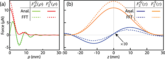
Figure 2. The disagreement of the forces calculated by analytical multipole expansion method (Anal., solid lines) and the more accurate numerical FFT method (FFT, dashed lines). (a) Force distribution on the radial axis and  . (b) Force distribution on the beam axis and
  .
.
Download figure:
Standard image High-resolution imageHere, we compared the decomposed force fields obtained through our FFT approach with those calculated using the analytical multipole expansion method. The multipole expansion method fails to accurately calculate the force fields in this case, because the truncated higher order multipoles are not negligible, and one must resort to the full Mie theory. To provide evidence for the accuracy of our force calculation method, we present the force fields of a spherical particle with a radius of 1 mm (λ = 8.7 mm) in appendix
3.2. GF and SF for focused acoustic beams
We begin by examining the GF and SF exerted on a polystyrene particle by the focused  acoustic beam. Due to the axial symmetry of the beam, the intensity distribution on the xy-plane (figure 3(a)) and xz-plane (figure 3(b)) can fully represent the focused beam in all space. The field of the beam center marked with green crosses is strong, meeting the rapidly decaying presumption specified by equation (1). As long as a sufficiently large 3D supercell is selected, such that the force acting on the particle decays to zero at the boundary, we can numerically compute GF and SF. The calculation of the acoustic force
  is based on the highly efficient and accurate Mie theory and translational addition theorem outlined in the appendix. After applying equation (1) to
  , we can obtain
  and
and  .
.

Figure 3. Intensity distribution of the focused acoustic beam with  in the xy-plane (a) and the xz-plane (b). The green crosses mark the coordinate center. a.u. denotes arbitrary unit.
Download figure:
Standard image High-resolution imageFor a spherical particle with a radius of 1 mm (shown in figures 4(a)–(f)) and 3 mm (shown in figures 4(g)–(l)) manipulated by  focused acoustic beam, the total force, GF, and SF are respectively given by
  ,
,  ,
,  . Since
  , no force depends on
  and
and  . Because of the axial symmetry, we only display the force in the ρz-plane, while the complete force can be obtained by revolving this plane. The force (both
  and
and  ) repel the particle away from the center, as expected for a solid particle located near the intensity maximum of the focused beam in air. On the other hand, the
  is not only the dominating component of SF, but also greater than GF near the beam axis, making stable trapping with
  impossible.
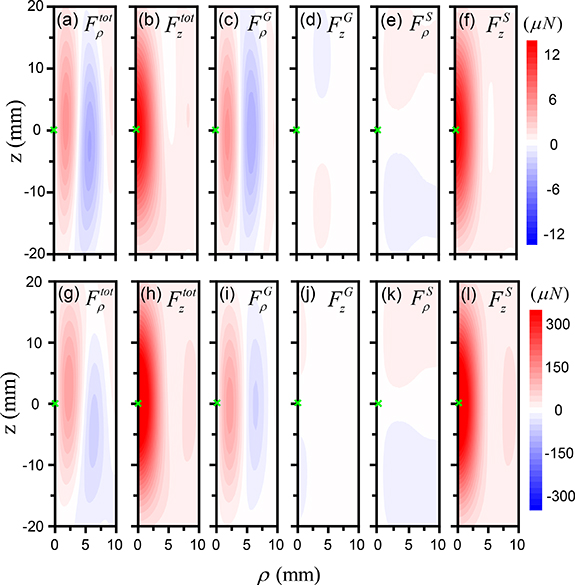
Figure 4. GF and SF for a spherical particle with a radius of 1 mm or 3 mm manipulated by a focused acoustic beam with  . Total force field
  (a), (b) for 1 mm-radius particle and (g), (h) for 3 mm-radius particle, GF
  (c), (d) for 1 mm-radius particle and (i), (j) for 3 mm-radius particle, and SF
  (e), (f) for 1 mm-radius particle and (k), (l) for 3 mm-radius particle in the ρz-plane.
Download figure:
Standard image High-resolution imageWe find that when the particle size increases from 1 mm-radius to 3 mm-radius, the SF will increase much more than GF. The profiles of both GF and SF are quite similar for particles with different sizes, indicating that they are mostly determined by the beam profile (intensity for GF and both intensity and phase for SF). However, their total forces are very different, because the relative strength of GF and SF varies with particle size. The symmetries in GF and SF are higher than that in the total force, indicating that these physically and mathematically distinct forces have hidden symmetries that are not revealed in the beam profile [42].
Figure 6 presented the GF and SF for a focused acoustic beam with  , where the particle radius is 1 mm and 3 mm. The intensities of
  beam in the xy-plane and xz-plane are shown in figure 5. With a nonzero
  , the azimuthal force SF emerges. The particle may be pushed near the focal plane due to the dominated GF, while the increased
  will rotate the particle around the propagation axis as long as it moves a little away from the beam axis. Meanwhile, along the beam axis, SF surpasses the GF in the longitudinal direction. Nevertheless, trapping along the axial direction may still be possible at an appropriate level of incident power, given that the mass of the particle can balance out the axial SF. We note that an angular momentum-carrying beam, such as those with nonzero
  , will drive the particle to rotate thus continuously transferring angular momentum and energy to the particle, and eventually allowing the particle to escape. For stable trapping, such angular momentum and energy have to be damped out by ambient damping, and it is not always possible, especially for large particles [65, 69].

Figure 5. Intensity distribution of the focused acoustic beam with  in the xy-plane (a) and the xz-plane (b). The green crosses mark the coordinate center. a.u. denotes arbitrary unit.
Download figure:
Standard image High-resolution image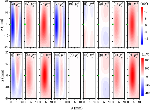
Figure 6. GF and SF for a spherical particle with a radius of 1 mm or 3 mm manipulated by a focused acoustic beam with  . Total force field
  (a)–(c) for 1 mm-radius particle and (j)–(l) for 3 mm-radius particle, GF
  (d)–(f) for 1 mm-radius particle and (m)–(o) for 3 mm-radius particle, and SF
  (g)–(i) for 1 mm-radius particle and (p)–(r) for 3 mm-radius particle in the ρz-plane.
Download figure:
Standard image High-resolution imageWhen the topological charge increases from  to
to  , the low-intensity region near the focus expands, and
  also increases accordingly, as shown in figure 7. When the particle is placed on the focal spot, it is almost free of the acoustic force. Nevertheless, it is not a stable equilibrium point, i.e. once the particle leaves a little distance away from the focus, it will escape from that area due to the off-centered transverse force.

Figure 7. GF and SF for a spherical particle with a radius of 1 mm manipulated by a focused acoustic beam with  . (a)–(b) Intensity distribution of the focused acoustic beam in the xy-plane (a) and the xz-plane (b). Total force field
  (c)–(e), GF
  (f)–(h), and SF
  (i)–(k) in the ρz-plane.
Download figure:
Standard image High-resolution imageIn acoustic trapping, the stability of the trapped particle is not solely determined by the conservative GF, which is typically designed to trap the particle at the center of the beam. On the other hand, SF also affects the stability of the trapped particle, but it cannot trap any particle by itself. For this reason, SF is commonly regarded as a force that undermines the stability of the trapped particle. In our study, we employ the FFT approach to decompose the total force field into GF and SF, allowing for a comparison between them. By examining the decomposed profiles of the GF and SF, one can gain a clearer understanding of how the trapped particle is manipulated in acoustic trapping. In the context of acoustic trapping using a focused beam, we have examined various topological charges ( ) and observed their significant impact on both the GF and SF profiles. As the topological charge goes non-zero, the GF turns the focus from a repulsive one to a trapping one. Nonetheless, the vortex-like SF aligned along the z-direction can still lead to the instability in trapping. Such observation aligns with the experiments in [65].
3.3. GF and SF for standing and non-standing wave fields produced by interfering PWs
Consider the interaction between a 5 mm-radius sphere and the acoustic PW fields in the xy-plane for a three-PW and a four-PW configuration. Figure 8(a) (figure 9(a)) shows three (four) equally angular PWs propagating on the xy-plane. The three-PW constitutes a non-standing field while the four-PW forms a standing field.

Figure 8. The acoustic radiation force field exerted on a 5 mm-radius spherical particle positioned in a three-beam acoustic plane wave is investigated. (a) The schematic of the three plane waves is shown. (b) Intensity distribution of the interfered plane waves in the xy-plane. Total force field  (c), (d), GF
  (e), (f), and SF
  (g), (h) in the xy-plane, where
  denote the coordinate of the particle in the xy-plane.
Download figure:
Standard image High-resolution image
Figure 9. The acoustic radiation force field exerted on a 5 mm-radius spherical particle positioned in a four-beam acoustic plane wave is investigated. (a) The schematic of the four plane waves is shown. (b) Intensity distribution of the interfered plane waves in the xy-plane. Total force field  (c), (d), GF
  (e), (f), and SF
  (g), (h) in the xy-plane, where
  denote the coordinate of the particle in the xy-plane.
Download figure:
Standard image High-resolution imageIn both kinds of fields, we plotted the acoustic intensity and particle forces in the xy-plane. The magnitude of the GF is a little larger than that of the SF in the non-standing field, and the SF completely vanished in the standing field. This indicates that SF is closely tied to the energy flux of the light, thus it takes a larger value in the non-standing field than in the standing wave case.
4. Conclusion
The total force for a millimeter-radius particle immersed in a 40 kHz acoustic field has been rigorously calculated and presented (within a square pillar domain). This total force field is then inputted to our FFT-based decomposition algorithm, where the conservative and nonconservative parts are separately computed. Nevertheless, FFT automatically assumes that the input force field is periodic. Therefore, while the FFT-algorithm has no problem with periodic sound field, non-periodic field will suffer from truncation error, and this error is tolerable only when the sound field is decaying sufficiently rapidly. There is a decreasing truncation error associated with increasing sample size. In appendix
For the focused beam configuration we considered, no zero-force position is found along the beam axis owing to the large pushing SF. Nevertheless, stable axial trapping is still possible since the particle mass can balance out the SF under appropriate conditions. GF and SF were found to be insensitive to particle size but depend strongly on the incident fields with different topological charges, as well as standing or non-standing waves.
The GF and SF also show symmetries that are not found in the total force or incident wave field. We conclude that this work may serve as a map for acoustic manipulation. One can select appropriate configurations to optimize or attenuate GF and SF to harmonize with specific applications.
Acknowledgments
This work was supported by Stable Support Plan Program of Shenzhen Natural Science Fund (Grant No. 20200925152152003), National Natural Science Foundation of China (Grant No. 12074169), and Guangdong Province Talent Recruitment Program (Grant No. 2021QN02C103). Huimin Cheng and Xixi Zhang contributed equally to this work.
Data availability statement
The data cannot be made publicly available upon publication because they are not available in a format that is sufficiently accessible or reusable by other researchers. The data that support the findings of this study are available upon reasonable request from the authors.
Appendix A: Mie theory
To obtain the acoustic force acting on a spherical particle, the radiation stress tensor is often applied (see appendix C), which requires the incident and scattered fields. The Mie theory offers a semi-analytic series solution to calculate the scattered fields for spherical particles [70–75]. We present a brief introduction to Mie theory.
The incident pressure field can be expanded as:

where  is the characteristic pressure amplitude,
  is the beam-shape coefficient (BSC) to be determined,
  is the nth order spherical Bessel function,
  is the spherical harmonic function of nth order and mth degree. The time dependence
  equation (A1) is omitted for the sake of simplicity, as we are calculating the time-averaged acoustic force exerted by a single-frequency wave.
In equation (A1), the incident field is expanded on the transducer's focus. To solve the acoustic scattering field, it is necessary to expand the incident field at center of the target sphere where the coordinates are  :
:

where  is the BSC about the coordinate system of
  [74]. Using the translational addition theorem, the translational BSCs are related to the original BSCs by a separation matrix
  :
:
Here  is a vector for the displacement of the coordinate origin,
  .
.
The scattered pressure field can be expanded similarly:

where  is the scattering coefficient, and
  is the nth order spherical Hankel function of first type. The scattering coefficient is determined by the boundary conditions [25], which states

where  is the pressure field inside the particle. After applying the boundary condition, one obtains

here  is the Mie coefficient given by

where  , and
, and  (
( ) and
) and  (
( ) are the density and wavenumber of the background medium (sphere), respectively. The apostrophe indicates the derivative with respect to the argument.
Appendix B: Focused beam and plane waves
B1. Focused beam field
The pressure amplitude in the focused beam field can be deduced from Rayleigh's integral, which performs the Huygens' principle and reveals that the pressure at a position  is the sum of wavelets generated on the surface of the transducer
  [73]:
[73]:

and  .
.  is the distance between an arbitrary point
  on the transducer's surface and the target point
  with
with  . The velocity distribution
  on the transducer surface in the configuration of the focused beam is defined by a pupil function:

Here,  and
and  are denoted in figure 1(a). The constant
  is the real amplitude of the vibration velocity. The topological charge
  denotes the phase variation, while the variation of polar angle is not taken into account by letting
  .
.
Meanwhile, the potential expression can be expanded using

with  . The incident pressure field can then be expressed as


Therefore, the BSC in pressure expansion is

B2. Plane wave field
A plane wave can be expanded as

where  represents the plane wave pressure field
  is the characteristic amplitude of pressure, both the plane wave vector
  and the position vector
  are expressed in a spherical coordinate system. Thus, BSCs for plane waves are

We remark that to move the coordinate center by  , it is sufficient to add a constant
  to every BSC:

Appendix C: Acoustic force calculation
We calculate the acoustic force by integrating the radiation stress tensor over the scatterer's surface. The time-averaged radiation stress tensor  is given by

where  stands for the time-average of the corresponding argument,
  and
and  is the identity matrix in three-dimension. The acoustic radiation force can be expressed by

where  is the characteristic energy density,
  ,
,  and
and  are the Cartesian unit vectors [74], and


where

Appendix D: Comparing the acoustic force obtained from Mie theory with other methods
Figure A10 depicts the y-direction force fields of a spherical particle with a radius of 1 mm (λ = 8.7 mm) as the particle's position varies along the x-axis. In this case, the particle is being manipulated by three coherent plane waves. The force values were determined using different methods: Mie theory (our method, indicated in red), multipole expansion (considering only monopole and dipole contributions, shown in green), the finite element method (COMSOL Multiphysics, shown in blue), and Multiple Scattering package in Julia language (an open-source program, shown in orange) [66–68]. Notably, the results obtained using Mie theory are consistent with those obtained using the finite element method and Julia language, but they differ from the results obtained using multipole expansion, which only accounts for monopole and dipole contributions. Evidently, the multipole expansion method, even with monopole and dipole contributions, has limitations in accurately calculating the 'total force', even for relatively small particles. To achieve accurate calculations of acoustic forces, it is necessary to include higher-order multipoles.

Figure A10. Acoustic force calculated by different methods. A 1 mm-radius particle is manipulated by three coherent plane waves (λ = 8.7 mm), as illustrated in (a). We show the y-direction force obtained by Mie theory (our method, red), dipole/monopole expansion (dipole/monopole, green), the finite element method (COMSOL Multiphysics, blue), and Multiple Scattering package in Julia language (an open-source program, orange).
Download figure:
Standard image High-resolution imageAppendix E: Verification of the numerical accuracy
In our approach, we utilize the fast Fourier transform (FFT) to decompose the total force field into two components: the conservative gradient force (GF) and the nonconservative scattering force (SF). It is required that the force field must exhibit either a 'rapidly decaying' or a 'periodic' behavior in order to be compatible with the FFT property.
In the case of a periodic force field, as long as the sampling points are sufficient, the resulting errors can be considered negligible. However, when dealing with a rapidly decaying force field, despite its rapid decay, the force field theoretically extends throughout the entire space. Therefore, in order to apply the FFT, it becomes necessary to 'truncate' the rapidly decaying force field using a 'box' domain, where the force field is sufficiently small outside its bounds. In our study, we used a cubic box domain with a volume  to truncate the force field.
Intuitively, the errors that arise are highly dependent on the size of the truncation box domain. The larger the box domain size (L), the smaller the resulting errors. In figure A11, we calculated and illustrated the decomposed SF using different L. It has been observed that a slight inconsistency exists between each case. However, it is important to note that the errors primarily occur near the boundaries of the box, where the discontinuity happens in the FFT technique. On the other hand, the force fields in the central region display a higher level of consistency across each case.

Figure A11. Scattering force versus the particle position on the z-axis for different truncation domains with L = 60 mm (black), L = 40 mm (red), L = 20 mm (blue), and L = 10 mm (pink).
Download figure:
Standard image High-resolution imageAppendix F: Numerical accuracy of the acoustic obtained from Mie theory
We note that the expansion series in the Mie theory are truncated with the empirical formula [76, 77]  , where
  and
and  represents the particle radius and wavenumber, respectively. In figure A12, we present the results of our simulations, demonstrating the acoustic forces exerted on a particle with a radius of 3 mm as the number of expansion series, N, increases. The dashed red line indicates the value of
  . Notably, it is observed that the force values converge before reaching
  , which shows that
  given by the empirical formula is sufficient to calculate the acoustic forces with a very high accuracy.

Figure A12. Acoustic force obtained from Mie theory versus the truncation order N. A focused beam with a topological charge m= 0 is considered. Different particle positions (a) (0, 0, 0)mm, (b) (1, 0, 0)mm, and (c) (1, 1, 0) mm are considered. The dashed line denotes the empirical truncation order we adopted, which is given by  , where
  and
and  denote the particle radius and the wavenumber, respectively.
Download figure:
Standard image High-resolution image