Efficient post-processing of electromagnetic plane wave simulations to model arbitrary structured beams incident on axisymmetric structures

The first principle behind our method lies in the angular spectrum approach for an electromagnetic field of angular frequency ω which can be expressed as,

$$\begin{equation} \mathbf{E}\left(\mathbf{r}\right) = \int^{2\pi}_{\phi = 0}\int^{\pi}_{\theta = 0} \mathcal{A}\left(\mathbf{k}\right) \, e^{i \, \mathbf{k} \cdot \left(\mathbf{r}-\mathbf{r}_0\right)} \, \underbrace{\textrm{sin}\left(\theta\right) \, \textrm{d}\theta \, \textrm{d}\phi}_{\textrm{d}\Omega_k}, \end{equation} \tag{ 1 }$$

where E is the electric field at a position $\mathbf{r} = (x,y,z)$, r₀ determines the phase centre of the optical field ¹ , $\mathcal{A}$ is the electric field's angular spectrum which is dependent on the wavevector $\mathbf{k} = k\big(\textrm{sin}(\theta) \, \textrm{cos}(\phi),\textrm{sin}(\theta) \, \textrm{sin}(\phi),$ $\textrm{cos}(\theta)\big)$, and $\Omega_k$ is the solid angle of the k-sphere defined by all possible orientations of k.

The angular representation indicates that any monochromatic electromagnetic field distribution can be decomposed into a linear combination of plane waves with varying spatial frequencies. One can be sure that any linear combination of plane waves will create another exact solution of Maxwell's equations and vice versa, any exact solution of Maxwell's equations (in linear materials) can be produced as a superposition of plane waves. We can further conceptualise the angular spectrum of any optical beam in free-space as a collection of plane waves that can all be mapped onto a single common propagating plane wave via some 3D rotations. This mapping is augmented by the angular spectrum in order to change the phase and magnitude of each plane wave as they are rotated. Instead of decomposing a known beam's field distribution, one can also conduct the inverse procedure, starting from a single plane wave, copy it a large number of times and both rotate and modulate the various copies according to the previously mentioned mapping. All the plane waves can be integrated and the resultant linear combination is equal to the desired optical beam.

If a spherical particle is added to the beam system, the fields are perturbed by the scattering. However, if we again take a single plane wave, this time incident on the spherical particle, and rotate the total vector field (complete with the sphere's scattering), we know that the solution is physically identical to the unrotated version because the particle is rotationally symmetric. Therefore with the simulation of a single plane wave incident on the spherical particle, we can repeat the process of rotating the fields and mapping the results to an angular spectrum of a beam, transforming this plane wave scattering system into the field distribution of a beam incident on the spherical particle. From this, we gain a strikingly general conclusion. Given a single simulation of a spherical particle with an incident plane wave, we can transform the plane wave into any optical illumination that we desire in simple post-processing steps. The rotational symmetry of the system reduces the number of required PWSs from infinite to just one. This is the second principle behind our method. Whilst this alone can still prove useful for simulating many common photonic systems, we can further extend this principle to cylinders, cones, tori, and any other particle shapes that possess continuous rotational symmetry (i.e. any axisymmetric body [48]) as follows.

We choose the convention that the particle is orientated such that an axis of rotational symmetry is along the z-axis (θ = 0) and a plane wave is incident at an azimuthal angle φ and an angle from the z-axis θ. The entire system can be rotated around the z-axis (i.e. varying the azimuthal angle φ) and still remain physically identical. However, any change in θ will not follow any symmetry in the system and so the scattering will be different. This indicates that a new simulation is needed for every value of θ, whilst all plane waves whom share the same value of θ are related to each other by a simple rotation about φ. We therefore need to sample a number of simulations with different values of θ to accurately extract the change in the scattering behaviour as θ changes. When compared with the general case where the particle has no symmetry at all and a large number of PWS would be required, we can still reduce the number of simulations needed significantly because the rotational symmetry effectively reduces the dimensionality of the problem.

Before we can apply symmetry arguments to simplify the problem, we must first be able to place particle scattering into a beam's fields via the angular spectrum approach. We can mathematically apply this to equation (1) by first expanding $\mathcal{A}$ into an orthogonal basis. We use a spherical polarisation basis with p/s naming conventions often used in surface optics. The $\hat{\mathbf{e}}_p(\mathbf{k})$ and $\hat{\mathbf{e}}_s(\mathbf{k})$ unit vectors correspond to the θ and φ unit vectors in spherical coordinates respectively. Details of this polarisation basis decomposition are provided in the supplementary information section 4. $\mathcal{A}(\mathbf{k})$ then splits into $A_p(\mathbf{k}) \, \hat{\mathbf{e}}_p(\mathbf{k}) + A_s(\mathbf{k}) \, \hat{\mathbf{e}}_s(\mathbf{k})$ and equation (1) becomes,

$$\begin{equation} \mathbf{E}\left(\mathbf{r}\right) = \iint \left[A_p\left(\mathbf{k}\right) \, \underbrace{\hat{\mathbf{e}}_p \, e^{i \, \mathbf{k} \cdot \mathbf{r}}}_{\textrm{plane wave}} +\, A_s\left(\mathbf{k}\right) \, \underbrace{\hat{\mathbf{e}}_s \, e^{i \, \mathbf{k} \cdot \mathbf{r}}}_{\textrm{plane wave}}\right] \, e^{-i \mathbf{k} \cdot \mathbf{r}_0} \, \textrm{sin}\left(\theta\right) \, \textrm{d}\theta \, \textrm{d}\phi. \end{equation} \tag{ 2 }$$

The scalar functions A_p and A_s are derived from $\mathcal{A}$ via dot products such that $A_p = \mathcal{A} \cdot \hat{\mathbf{e}}_p$ and $A_s = \mathcal{A} \cdot \hat{\mathbf{e}}_s$. Equation (2) explicitly highlights which terms correspond to plane waves of each polarisation state because these are the terms that PWS fields can replace via substitution to incorporate particle scattering into the beam fields $\mathbf{E}(\mathbf{r})$. That is to say, $\mathbf{E}(\mathbf{r})$ transitions from the free-space beam to a beam incident on a scattering structure when $\hat{\mathbf{e}}_{p,s} \, e^{i \, \mathbf{k} \cdot \mathbf{r}} \to \mathbf{E}_{p,s}^{\textrm{PWS}}(\mathbf{r};\mathbf{k})$. The vector field $\mathbf{E}_{p,s}^{\textrm{PWS}}(\mathbf{r};\mathbf{k})$ is the PWS calculated over real space (r) but it also varies with k (i.e., with θ and φ) because it represents the material structure being illuminated by a plane wave of all possible orientations. Given that the individual PWS (if computed correctly) comply with all Maxwell boundary conditions, the linearity of the equations guarantee that the synthesised structured illumination will comply with all boundary conditions too. Symmetry arguments can then be applied to $\mathbf{E}_{p,s}^{\textrm{PWS}}(\mathbf{r};\mathbf{k})$ to greatly reduce the number of simulations required and instead implement a series of computationally cheap 3D rotations to map a small number of simulations to all possible $\mathbf{E}_{p,s}^{\textrm{PWS}}(\mathbf{r};\mathbf{k})$.

The final step before numerical implementation is to discretise the continuous integrals over θ and φ into finite sums, and we arrive at the fundamental expression for numerically generating the fields of an arbitrarily structured beam incident on a material structure,

$$\begin{equation} \mathbf{E}\left(\mathbf{r}\right) \approx \sum_{p,s} \sum_\theta \sum_\phi A_{p,s}\left(\mathbf{k}\right) \, \mathbf{E}_{p,s}^{\textrm{PWS}}\left(\mathbf{r};\mathbf{k}\right) \, e^{-i \, \mathbf{k} \cdot \mathbf{r}_0} \, \textrm{sin}\left(\theta\right) \, \Delta \theta \, \Delta \phi. \end{equation} \tag{ 3 }$$

The first of the three summations indicate a sum over the two polarisation states p and s. The latter two sum over the plane wave orientations in spherical coordinates.

In some cases, it is desirable to simulate the scenario where the symmetric particle is not located at the beam's focus. A common example of this would be for doughnut beams where the focus has a low electric field intensity. In this case, optical forces due to the electric field intensity are likely stronger away from the focus of the beam. The $e^{-i \, \mathbf{k} \cdot \mathbf{r}_0}$ term allows for the translation of the beam's focus without the need for recalculations of $\mathbf{E}_{p,s}^{\textrm{PWS}}(\mathbf{r};\mathbf{k})$ by changing the relative phases of different PWS components. This allows for the efficient creation of informative graphs such as a force maps, in which the optical force is plotted as a function of the particle position within the beam, in a post-processing manner. This is demonstrated in section 3.2.

One of the key features of this method lies in its ability to rapidly compute a wide range of illumination types from the same numerical simulation data files. In the case where a numerical solver is capable of illuminating an object with a sophisticated beam structure (more than a single plane wave), any change in the beam parameters such as angle of incidence, focus position, beam waist and polarisation will always necessitate a completely new and potentially costly simulation. Any parameter sweeps will therefore be computationally expensive. Our method requires a minimal number of preliminary numerical simulations with plane waves and then manipulates this minimal data to achieve any illumination structure. Crucially, this allows for parameter sweeps such as angle of illumination or translating the beam's focal point to be performed efficiently by post-processing the same initial PWSs.

We shall now discuss how an incident beam field can be expressed with the angular spectrum and implemented in our approach, but we emphasise that the angular spectrum representation is not limited to beam structures; any electromagnetic field incident on an object can be represented with the angular spectrum approach using equation (1). Optical beams are often expressed in their paraxial approximation forms to simplify calculations [49] but in doing so, one loses both an exact solution to Maxwell's equations and some physical properties related to focusing such as a longitudinal field component [50–56]. We do not wish our method to suffer from these limitations. To rectify this, one can use the angular spectrum approach to begin with a paraxial equation and then determine the longitudinal component to create a 3D field distribution that obeys the laws of electromagnetism in all regimes and across all of space. This is possible because the angular spectrum is based on a linear combination of plane wave solutions, and each plane wave is an exact solution of Maxwell's equations. To do this, we implement the following procedure.

2.2.1. Integrating a paraxial beam

We begin with the fields of a paraxial beam with a propagation axis denoted by $\hat{\mathbf{K}}$. To start our argument, lets restrict the propagation to the z-axis (i.e. $\hat{\mathbf{K}} \parallel \hat{\mathbf{z}}$) and only require the fields in the focal plane, which we specify as z = 0. The paraxial field is therefore denoted by $\mathbf{E}_\perp^{\hat{\mathbf{K}} \parallel \hat{\mathbf{z}}}(x,y,0)$, where the $\perp$ symbol indicates that the fields are only polarised in the plane transverse to the propagation direction. The fields of the beam may be defined in Cartesian coordinates so it is convenient to recast equation (1) into the Cartesian basis with $\mathbf{k} = (k_x,k_y,k_z)$,

$$\begin{equation} \mathbf{E}_\perp^{\hat{\mathbf{K}} \parallel \hat{\mathbf{z}}}\left(x,y,0\right) = \underset{k_x^2+k_y^2 \unicode{x2A7D} k^2}{\iint}\mathcal{F}_\perp^{\hat{\mathbf{K}} \parallel \hat{\mathbf{z}}}\left(k_x,k_y\right) \, e^{i\left(k_x \, x + k_y \, y\right)} \, \textrm{d}k_x \, \textrm{d}k_y. \end{equation} \tag{ 4 }$$

Here $\mathcal{F}$ denotes the angular spectrum, but defined on the 2D z = 0 plane rather than a sphere dictated by θ and φ (refer to the supplementary information for more details). We relate $\mathcal{F}$ to the $\mathcal{A}$ that appears in equation (1) later in this procedure. The inverse of this Fourier transform is,

$$\begin{equation} \mathcal{F}_\perp^{\hat{\mathbf{K}} \parallel \hat{\mathbf{z}}}\left(k_x,k_y\right) = \frac{1}{4 \pi^2} \overset{\infty}{\underset{-\infty}{\iint}} \mathbf{E}_\perp^{\hat{\mathbf{K}} \parallel \hat{\mathbf{z}}}\left(x,y,0\right) \, e^{-i\left(k_x \, x + k_y \, y\right)} \, \textrm{d}x \, \textrm{d}y. \end{equation} \tag{ 5 }$$

For a simple paraxial Gaussian beam centred at the origin, $\mathbf{E}_{\perp}^{\hat{\mathbf{K}} \parallel \hat{\mathbf{z}}}(x,y,0) = (E_x,E_y,0) \, e^{-\frac{x^2+y^2}{w^2}}$, where w is the beam waist, and E_x and E_y are complex scalars that determine the phase, amplitude and polarisation of the beam's transverse field [46, 57–60], the corresponding angular spectrum would be $\mathcal{F}_\perp^{\hat{\mathbf{K}} \parallel \hat{\mathbf{z}}}(k_x,k_y) = (E_x,E_y,0) \, w^2 \, e^{-\frac{w^2}{4}(k_x^2 + k_y^2)}$. This step can be streamlined by referring to the table in the supplementary information section 3 which lists forms of $\mathcal{F}_\perp^{\hat{\mathbf{K}} \parallel \hat{\mathbf{z}}}$ for some common beam modes.

2.2.2. Extending from focal plane to all space

To extend the fields on the z = 0 plane from equation (4) to all space, we specify that the exact field E (which we wish to compute in the end) must fulfil the wave equation $\mathbf{k} \cdot \mathbf{k} = k^2$ and consists of only propagating components ($k_x^2+k_y^2 \unicode{x2A7D} k^2$). This leads to the propagator $e^{i k_z z}$ where $k_z = \sqrt{k^2-k_x^2-k_y^2}$ and $k_z\gt0$. The field can therefore be extended to all space via this propagator so that,

$$\begin{equation} \mathbf{E}_\perp^{\hat{\mathbf{K}} \parallel \hat{\mathbf{z}}}\left(\mathbf{r}\right) = \underset{k_x^2+k_y^2 \unicode{x2A7D} k^2}{\iint} \mathcal{F}_\perp^{\hat{\mathbf{K}} \parallel \hat{\mathbf{z}}}\left(k_x,k_y\right) \, e^{i \mathbf{k} \cdot \mathbf{r}} \, \textrm{d}k_x \, \textrm{d}k_y.\end{equation} \tag{ 6 }$$

2.2.3. Correcting for longitudinal fields

$\mathcal{F}_\perp^{\hat{\mathbf{K}} \parallel \hat{\mathbf{z}}}$ only has components $(\mathcal{F}_x,\mathcal{F}_y,0)$ in the transverse plane and lacks a longitudinal field component, owing to the fact that it is derived from a paraxial field. Now consider the field:

$$\begin{equation} \mathbf{E}^{\hat{\mathbf{K}} \parallel \hat{\mathbf{z}}}\left(\mathbf{r}\right) = \underset{k_x^2+k_y^2 \unicode{x2A7D} k^2}{\iint} \mathcal{F}^{\hat{\mathbf{K}} \parallel \hat{\mathbf{z}}}\left(k_x,k_y\right) \, e^{i \mathbf{k} \cdot \mathbf{r}} \, \textrm{d}k_x \, \textrm{d}k_y. \end{equation} \tag{ 7 }$$

This is the full true Maxwell field including longitudinal components, with no approximation, and its only condition being that its transverse components match $\mathbf{E}^{\hat{\mathbf{K}} \parallel \hat{\mathbf{z}}}_\perp(\mathbf{r})$. Explicitly, $\mathcal{F} = \mathcal{F}_x \hat{\mathbf{x}} + \mathcal{F}_y \hat{\mathbf{y}} + \mathcal{F}_z \hat{\mathbf{z}}$ whilst $\mathcal{F}_\perp = \mathcal{F}_x \hat{\mathbf{x}} + \mathcal{F}_y \hat{\mathbf{y}}$. The missing component can be retrieved by invoking Maxwell's equation $\mathbf{\nabla} \cdot \mathbf{E} = 0$ and applying it to equation (7) to obtain the condition $\mathbf{k} \cdot \mathcal{F} = 0$. This condition explicitly states that $k_x \, \mathcal{F}_x + k_y \, \mathcal{F}_y + k_z \, \mathcal{F}_z = 0$ and so,

$$\begin{equation} \mathcal{F}_z = -\frac{\mathcal{F}_x \, k_x + \mathcal{F}_y \, k_y}{k_z}. \end{equation} \tag{ 8 }$$

This is to say that when the fields in the transverse plane are known, the longitudinal field can be easily reconstructed using this simple equation and turns $\mathcal{F}_\perp^{\hat{\mathbf{K}} \parallel \hat{\mathbf{z}}} \to \mathcal{F}^{\hat{\mathbf{K}} \parallel \hat{\mathbf{z}}}$. For our Gaussian beam example, this results in $\mathcal{F}^{\hat{\mathbf{K}} \parallel \hat{\mathbf{z}}}(k_x,k_y) = (E_x,E_y,E_z) \, w^2 \, e^{-\frac{w^2}{4}(k_x^2 + k_y^2)}$, where $E_z = -\frac{E_x \, k_x + E_y \, k_y}{k_z}$.

2.2.4. Defining a piecewise angular spectrum

Since equation (2) computes the integration of $\mathcal{A}$ over the surface of a 3D sphere and equation (7) integrates $\mathcal{F}$ over the 2D z = 0 plane when $k_z\gt0$, $\mathcal{F}$ must be related to $\mathcal{A}$ with a piecewise mapping and accounting for the different Jacobians in the integrals. The differential solid angle $\textrm{d}\Omega = \textrm{sin}(\theta) \, \textrm{d}\theta \, \textrm{d}\phi = \frac{1}{k \, k_z} \, \textrm{d}k_x \, \textrm{d}k_y$ [46] and results in,

$$\begin{equation} \mathcal{A}^{\hat{\mathbf{K}} \parallel \hat{\mathbf{z}}}\left(\mathbf{k}\right) = \begin{cases} k \, k_z \, \mathcal{F}^{\hat{\mathbf{K}} \parallel \hat{\mathbf{z}}}\left(k_x,k_y\right), & \textrm{if} \,\, k_z > 0 \\ 0, & \textrm{if} \,\, k_z \unicode{x2A7D} 0. \end{cases} \end{equation} \tag{ 9 }$$

For our simple Gaussian beam example, this indicates that $\mathcal{A}^{\hat{\mathbf{K}} \parallel \hat{\mathbf{z}}}(\mathbf{k}) = (E_x,E_y,E_z) \, k \, k_z \, w^2 \, e^{-\frac{w^2}{4}(k_x^2 + k_y^2)}$.

2.2.5. Rotation of beam axis

2.2.6. Obtaining non-paraxial 3D fields

When a beam is incident on a particle, it can manipulate its position and orientation via optical forces and optical torques. These phenomena are driven by the transfer of linear and angular momentum from the beam to the particle respectively, and can be readily calculated from 3D electromagnetic field data via the Maxwell stress tensor (MST) method. The MST, denoted by $\overset\leftrightarrow{\mathbf{T}}$, represents the flow of momentum in the field and can be expressed as [46],

$$\begin{equation} \langle\overset\leftrightarrow{\mathbf{T}}\rangle = \frac{1}{2} \mathfrak{Re} \left\{\varepsilon \mathbf{E} \otimes \mathbf{E}^* + \mu \mathbf{H} \otimes \mathbf{H}^* - \frac{1}{2} \left(\varepsilon |\mathbf{E}|^2 + \mu |\mathbf{H}|^2\right)\overset\leftrightarrow{\mathbf{I}}\right\}, \end{equation} \tag{ 10 }$$

where E and H are the total electric and magnetic fields, ⊗ denotes the outer product of two vectors, asterisks represent complex conjugations, $\overset\leftrightarrow{\mathbf{I}}$ is the $3 \times 3$ identity matrix and ε and µ are the permittivity and permeability of the medium, respectively. The angular brackets indicate a time-averaged quantity. A force occurs when there is a net inward or outward flow of momentum into the body experiencing the force and can be quantified by the flux surface integral [46],

$$\begin{equation} \langle\mathbf{F}\rangle = \int_{S}^{} \langle\overset\leftrightarrow{\mathbf{T}}\rangle \cdot \hat{\textbf{n}} \, \textrm{d}S, \end{equation} \tag{ 11 }$$

where F is the optical force and $\hat{\textbf{n}}$ is the outward normal vector of any arbitrary closed surface S enclosing the body. Likewise, the torque can be calculated by imposing the definition of angular momentum with a cross product such that,

$$\begin{equation} \langle\mathbf{N}\rangle = \int_{S} \left(\mathbf{r} \times \big\langle\overset\leftrightarrow{\mathbf{T}}\big\rangle \right) \cdot \hat{\textbf{n}} \, \textrm{d}S, \end{equation} \tag{ 12 }$$

where N is the optical torque and r is the position vector from the axis of rotation. The collective cross product term in the brackets is sometimes referred to as the angular momentum flux tensor [61, 62]. With these expressions, one can immediately determine particle dynamics originating from electromagnetism regardless of the particle's properties. The only quantities required to calculate forces and torques from equations (11) and (12) are the full electromagnetic fields (both electric and magnetic) of the incident beam scattering on the particle, which our method provides.

Multilayered spherical particles are a common solution when a particle's scattering/absorption needs to be engineered. Such particles can be fabricated with modern nanofabrication techniques [63] and have been proposed for applications including photocatalysis, nanolasers, spontaneous emission enhancement and as a basis for nonlinear phenomena. In this example, we use the gold-core silicon-shell design outlined by Feng et al [64] which exhibits a pure magnetic dipole resonance at a wavelength of $\lambda = 1.3 \, \mu\mathrm{m}$. This core–shell particle therefore probes the magnetic field of any incident beam. The core radius is 62 nm and the shell radius is 180 nm. The rotational symmetry of this geometry means that only two PWS are needed (one for each polarisation) in order to calculate the interaction between a multilayered sphere and a beam of any structure.

Figure 1(b) shows a schematic of the system with the beam propagating along the positive z-axis. The beam waist w is set to 0.5λ where $\lambda = 1.3 \, \mu\mathrm{m}$, and the surrounding medium has n = 1. After a very quick simulation of two PWSs scattering on the particle in CST Microwave Studio, our post-processing code was applied to them. The output is the full fields for an incident circularly polarised tightly focused Gaussian beam scattering on the core–shell particle. The angular spectrum of this illumination is conveniently provided by the package's analytical workbook. Figure 1(c) shows a cross section of $|\mathbf{E}|$ in the y = 0 plane and the particle is outlined with a black dotted line. The interference between the incident beam and the particle's scattering is clearly visible in the bottom half of the image. This 3D electromagnetic field distribution was used to calculate the optical force and torque on the particle using the MST method. A cubic surface enclosing the particle was chosen for the integration. In principle, any size of this cube enclosing the particle should result in the same force and torque. Numerically, however, there are always variations, so it is important to check consistency and obtain a statistically accurate value for these quantities by varying the size of the integration surface (see figure 1(d)). Figure 1(d) shows the Cartesian components of the force and torque calculated across a range of integration cube sizes, and flat lines indicate a reliable result. The yellow region (a < 360 nm) indicates where the integration surface is too small and intersects with the particle, resulting in inaccurate results.

Zoom In Zoom Out Reset image size

A spherical particle is a special case in scattering problems because Mie theory provides an exact analytical solution to the problem. Therefore, we can evaluate the accuracy of our numerical method by comparing with the results obtained through Mie theory. The details of these analytical calculations are provided in the supplementary information, and the theoretical values for the force and torque (denoted by $F_\textrm{th}$ and $N_\textrm{th}$) are plotted in figure 1(d) with blue and orange dotted lines, respectively. We observe a strong agreement between theoretical and numerical results, indicating a reliable numerical calculation.

This example used a core–shell particle with a single shell, but we note that the method is applicable to any geometry with the required symmetry, hence any number of shells could be applied in this methodology. When attempting to recreate a real system from the laboratory, experimental tolerances in the fabrication of core–shell particles should be accounted for in the PWS. For example, one can conduct parameter sweeps of critical parameters such as particle dimensions and surface roughness. Any additional effects such as doping should be accounted for in the optical properties of the materials when performing the PWS.

As described in detail above, we could now vary any parameter of this beam (waist, size, focus location, type of beam, etc) and simply run the post-processing steps on the same two PWS to obtain the new fields, force and torque.

The next phase in this demonstration is the use of sophisticated structures that are more difficult to solve. Without spherical symmetry, analytical methods such as Mie theory no longer provide an immediate answer to the scattering problem. Cylinders are commonplace in nanophotonics [41] but cylindrical symmetry applies to a far wider range of geometries than just cylinders; structures such as cones [65, 66], tori/rings [67–70], tubes and core–shell cylinders [38] are examples of this. Out of these structures, a conical geometry is perhaps one of the most difficult to calculate because it lacks the cross-sectional mirror symmetry that would enable a further reduction in the number of PWS from $0 \unicode{x2A7D} \theta \unicode{x2A7D} \pi$ to $0 \unicode{x2A7D} \theta \unicode{x2A7D} \frac{\pi}{2}$. For this reason, the next example uses a nanocone.

Gold nanocones are already experimentally viable and the plasmonic nature enables stronger scattering [65]. The illuminating beam's complexity has also been increased by selecting a focused azimuthally polarised vortex beam to emphasise the range of possible beam options. Furthermore, the angle of incidence is set to 45^∘ and the focal point has been displaced away from the nanocone to highlight that the beam axis can be chosen independently of the cylindrical symmetry axis. The wavelength is set to 532 nm to match the plasmonic resonance range of gold, and the beam waist is set to 0.8 λ. Once again, PWS were carried out in CST Microwave Studio for plane waves incident on the nanocone at different angles of incidence θ (but always keeping φ = 0). This PWS data was then post-processed using our code to obtain the full field distributions under the desired incidence.

Figure 2(a) shows the y = 0 cross-section plane of the beam's electric field distribution in free-space and figure 2(b) introduces the gold nanocone to the beam at the point of highest intensity. The nanocone has a height of 240 nm and a maximum radius of 50 nm. Similar to figure 1(b), we clearly observe the nanocone's scattering interfering with the incident beam and further see a hot spot at the base of the cone. This hot spot agrees with previous results in literature [65] where a similar excitation is seen with the same material and a similar wavelength. Figure 2(c) shows the optical force and torque on the nanocone and is analogous to figure 1(c). The force is directed along the beam's propagating direction so can be explained as a simple radiation pressure on the nanocone. F_z is also slightly larger than F_x , suggesting that the nanocone's hot spot is being pushed towards the maximum of the beam. The torque along the −y direction indicates that the nanocone will rotate anti-clockwise from figure 2(b)'s perspective. Further iterative calculations could be conducted in order to determine an orientation with rotational equilibrium.

Zoom In Zoom Out Reset image size

Finally, in order to highlight the method's power and without requiring additional PWSs, we applied the post-processing code to sweep the nanocone position across the beam by changing r₀ in equation (3) and calculated a force map shown in figure 2(e). Each arrow in this figure represents a full post-processing simulation each including MST integration in a cube around the particle. Producing a force map would have been a tedious process if performing individual numerical simulations for each nanocone position, but we can use our approach to create such a plot in a matter of minutes on a standard desktop computer, all from the same set of PWS.

The previous examples focused on standalone particles, but this calculation method is equally valid for configurations involving planar structures. A planar interface is naturally axisymmetric and so rotations around the surface's normal axis yield physically identical results and therefore can be exploited to reduce the dimensionality of the problem. A multilayered or stratified structure is merely an extension of this problem and can be calculated in a similar manner to the previous examples by also applying the well-established transfer matrix method [71].

We demonstrate this case with a p-polarised focused vortex beam (Laguerre–Gaussian with l = 1 and m = 0) reflecting off of a glass-gold multilayered structure, and the resulting electric field distribution is portrayed in figure 3. The beam has a wavelength of 808 nm and is focused at the origin to a beam waist of 0.75λ. The glass, with a refractive index of 1.5, is 1 µm thick and semi-infinite gold [72] is placed beneath it. The incident polarisation singularity is clearly visible along the $z = -x$ line and an interference pattern is observed around the air-glass interface.

Zoom In Zoom Out Reset image size

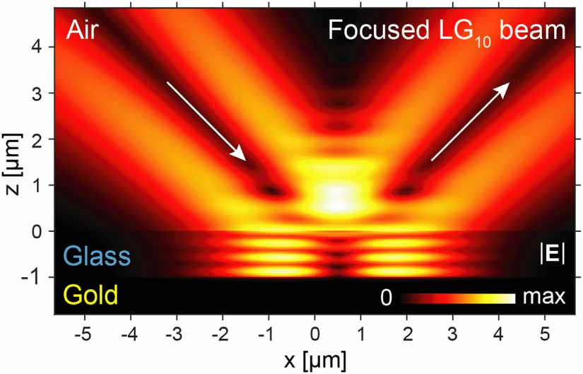
The 3D electromagnetic fields were calculated in figure 3 using both a commercial frequency-domain numerical solver with periodic Floquet boundary conditions and with an analytical calculation of the multilayer scattering of plane waves. The latter is naturally faster computationally but is limited to homogeneous layered systems. Numerical solvers enable the calculation of more complicated axisymmetric structures such as an isolated nanorod or nanocone on a substrate, or a recess like an isolated nanopore. Whilst these structures are regularly found within tightly packed periodic metamaterials, the isolated structure results still provide valuable information about the structure's resonant behaviour under complex beam illumination, and how the substrate augments these properties. In this way, we expect our package to prove a valuable tool for experimental groups looking to gain a deeper understanding of their experimental nanomaterials that consist of these elements when illuminated with a complex beam. In the event where the rod/cone/pore separations are large enough for neighbouring element interactions to become negligible, this axisymmetric angular spectrum approach will yield approximate quantitative results.