


Abstract
We theoretically investigated frustrated tunneling ionization (FTI) driven by spatially inhomogeneous strong laser fields induced by surface plasmon resonance within a bow-tie metal nanostructure. The results show that the FTI probability and the principal quantum number distribution exhibit similar oscillatory behavior as a function of the pulse duration. Our analysis reveals that the periodic defocusing and refocusing of the electron spatial distribution due to the inhomogeneous laser field is responsible for the oscillatory structures. In addition, the initial tunneling coordinates and the angular momentum distributions of the FTI events and theirs pulse duration dependence are also explored. Moreover, our results show that the frequency of the oscillatory structures depends sensitively on the electron quiver amplitude and the inhomogeneity strength. Thus, the electron quiver amplitude and the size of the gap between bow-tie nanostructure are useful and efficient knobs for controlling the yield and properties of exited Rydberg states.
Export citation and abstract BibTeX RIS

Original content from this work may be used under the terms of the Creative Commons Attribution 4.0 license. Any further distribution of this work must maintain attribution to the author(s) and the title of the work, journal citation and DOI.
1. Introduction
Tunneling ionization is a fundamental physical process in the interaction of an ultra-short intense laser pulse with atoms or molecules. If the field strength of laser field becomes comparable to the binding Coulomb force, the outermost electron of atoms or molecules can be released into the continuum via tunneling ionization. Subsequently, the tunneled electron may be pulled back by the oscillating laser electric field, and then scattered by the parent ion [1], resulting in all sorts of highly nonlinear phenomena, such as high harmonic generation (HHG) [2, 3], above-threshold ionization (ATI) [4, 5], nonsequential multiple ionization [6–8], and photoelectron holography [9–13].
Besides, even when driven by such strong laser pulses, a considerable fraction of electrons can still survive in high-lying Rydberg states [14–28]. The underlying physical mechanism for the generation of excited Rydberg state which is known as frustrated tunneling ionization (FTI) process has been identified experimentally and theoretically, that is, the drift energy obtained by the ionized electron in the subsequent electric field is too small to escape from the Coulomb force of the ion, and eventually the electron is recaptured into highly excited state at the end of the laser pulse [14]. This FTI scenario has not only successfully reproduced the principal quantum number distribution of the generating Rydberg states and the dependence of the yield of Rydberg state on the ellipticity of the laser pulse [14, 15], but also initiated various applications, such as strong-field acceleration of neutral particles [16], precision measurements [17], and generation of coherent extreme-ultraviolet emission [18, 19] etc.
The laser field governs the movement of the ionized electron after tunneling. Thus, by adjusting the parameters of the laser field, one can effectively control the microscopic electron dynamics in the FTI process and manipulate the properties of Rydberg states [19–25]. Recently, the spatially structured field, i.e. the optical near field when a laser pulse is illuminated on a nanostructure [29–43], has attracted much interesting in control the electron dynamics in strong laser field. The laser field undergoes an exponential increase in intensity as the ionized electron moves closer to the nanotips. At this time, the influence of the strong spatial inhomogeneity on the movement of the electron can be described by the parameter  , where
  is the decay length of the laser field and
  is the electron quiver amplitude [29]. Compared with that in a homogeneous field, the ionized electron can obtain greater returning energy in the inhomogeneous field. This characteristic has attracted extensive attention, especially for HHG and ATI. For example, driven by the inhomogeneous field, the ionized electron can be accelerated to a high energy near the KeV regime [30], resulting in a significant extension of the harmonic cutoff [31–33]. Moreover, due to the asymmetry of the total potential, the odd and even harmonics can be generated simultaneously [32, 33]. In ATI, the spatial inhomogeneity can result in the higher-energy structure in the photoelectron energy spectrum [34]. The underlying electron dynamics process driven by the inhomogeneous field has been revealed with the classical trajectory or quantum orbital model [34–37].
In this work, we theoretically study FTI within spatially inhomogeneous field induced by a bow-tie nanostructure. The results show that FTI probability and principal-quantum-number distribution exhibit interesting pulse-duration-dependent oscillations. Our analysis shows that the periodical defocusing and refocusing of the spatial distribution of tunneling electrons during the propagation lead to oscillations of the final energies of electron and the final distances of electrons to the ion core, giving rise to the observed oscillatory structures. In addition, the initial tunneling coordinates  and the angular momentum distributions of the FTI events and theirs pulse duration dependence are also explored. Moreover, our results indicate that the period of the oscillation of the FTI yield depends on the electron quiver amplitude and the inhomogeneity strength.
2. Methods
To simulate the FTI process driven by spatially inhomogeneous laser pulses induced by a bow-tie metal nanostructure, a classical-trajectory Monte Carlo (CTMC) model is employed. This CTMC model, which has had tremendous success in investigating electron dynamics in numerous strong-field phenomena [19–21], provides physically intuitive insights into the underlying mechanism by tracing back the classical electron trajectories. In accordance with prior studies, the FTI process can be divided into two steps: tunneling ionization and classical propagation.
In the tunneling ionization step, the outermost electron tunnels through the field-suppressed Coulomb potential with a zero initial longitudinal momentum parallel to the laser polarization direction and a Gaussian-like initial transverse momentum distribution perpendicular to the laser polarization direction. The tunneling exit is given by  [20, 24]. Each electron trajectory is weighted by the ADK ionization rate (in this work we employ atomic units unless stated otherwise):

where  is the tunneling time,
  is the initial transverse momentum,
  is the instantaneous electric field strength at the instant
  of tunneling, and
  a.u. is the ionization potential of our model atom which is equal to that of Ar atom. In our calculations, the ensemble is obtained by sampling 6 million of classical trajectories. In our calculations, the ensemble of classical trajectories are sampled over the tunneling ionization time
  , where T is the optical cycle of the laser field. This type of sample facilitates demonstration of the physics in this work. In the real femtosecond pulses, tunneling ionization of the first electron is mainly concentrated within a few half optical cycles around the peak of the pulse. In this case, the phenomenon demonstrated in the following will not less obvious but still survives.
In the classical propagation step, the evolution of the electron's trajectory is governed by the Newton's classical motion equations:

where  is the ion core-electron potential energy, and we set the softening parameter
  to avoid the Coulomb singularity. An FTI event occurs when an electron acquires negative energy (the total energy as the sum of kinetic energy and Coulomb potential) after the laser field is removed. This work we focus on the principal quantum number and the angular momentum distributions of the electron lying on the Rydberg state. The principal quantum number is calculated by
  , and the angular momentum is calculated by
  , where
  ,
,  and
and  are the energy, position and momentum of the electron lying on the Rydberg state at the end of the laser pulse, respectively [14, 21].
In this work, the spatially inhomogeneous field generated by bow-tie nanostructures is written as:

where  is the peak amplitude of the laser electric field,
  a.u. is the frequency of the 800 nm laser field and
  is the trapezoidal pulse envelope which has N optical cycles in total with the last two optical cycles ramping off. Furthermore,
  represents the parameter characterizing the inhomogeneity strength.
The bow-tie nanostructure takes the form of two identical triangular-shaped gold pads separated by a finite gap, and the schematic illustration of its geometric structure is shown in figure 1(a). In our simulations, we set the longest altitude  to be 600 nm, the smallest acute angle to 30◦, the thickness of the pads to 25 nm and the gap
  between two tips to 30 nm. Considering the limitation of current machining techniques and to avoid the enhancement of the nonphysical fields by tip-effect, we set the curvature radii of the tips as 10 nm.
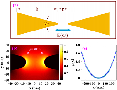
Figure 1. (a) Schematic diagram of geometric structure of the bow-tie gold nanostructure. (b) The relative intensity enhancement in the gap region of the bow-tie nanostructure. (c) The functional form of the inhomogeneity strength parameter  . The circles are the raw data obtained from the FDTD simulations and the blue line is an interpolation fitting.
Download figure:
Standard image High-resolution imageThe electric field intensity enhancement inside the gap of the bow-tie nanostructure was numerically calculated by the finite difference time domain method (FDTD), using the Au (gold)—CRC optical property. Figure 1(b) displays the relative enhancement of the electric field intensity in the gap of the bow-tie nanostructure when irradiated by a linearly polarized laser pulse with a wavelength of 800 nm for  = 30 nm. The polarization direction of the laser field is along the x axis. The enhancement profile of the electric field intensity is extracted along the bow-tie nanostructure long axis through the middle of the gap. Figure 1(c) shows the functional form of the inhomogeneity strength parameter
  with respect to the position inside the gap of the bow-tie nanostructure, where the circles are the raw data obtained from the FDTD simulations and the blue line is an interpolation fitting. Note that in the classical propagation step, all atoms are initially located at the center of the bow-tie nanostructure along x-axis (that is
  ). If the initial position of an atom is randomly distributed between the bow-tie nanostructure, it means the inhomogeneity strength parameter is randomly given, and therefore the results shown below will be weaken or obscured. However, in the real experiment, the atoms in a gas jet should obey the Gaussian distribution but not random distribution.
3. Numerical results and discussions
3.1. Pulse duration dependence of FTI in the inhomogeneous fields
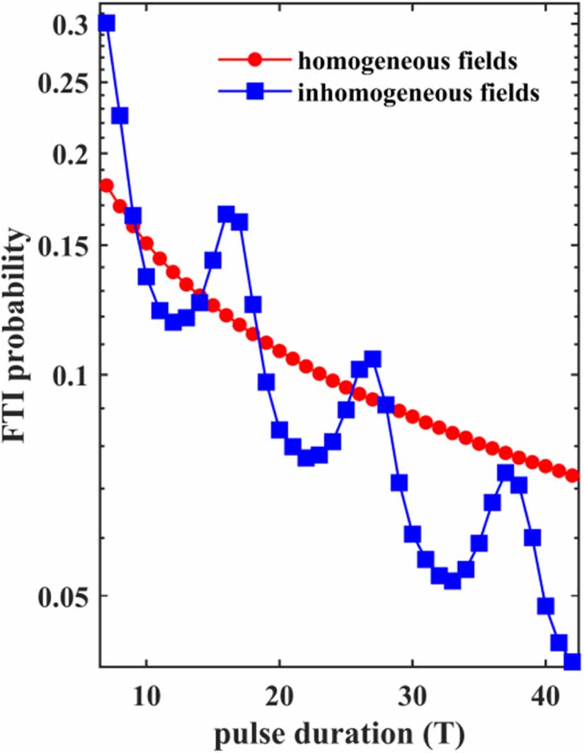
Figure 2 displays the probabilities of FTI as a function of laser pulse duration in the term of number of optical cycle N. The red dotted-line and blue squared-line represent the case of spatially homogeneous and inhomogeneous laser field respectively. It is shown that for homogeneous field, the FTI probability decreases monotonously as pulse duration increases. This is consistent with previous theoretical predictions [19, 21]. For inhomogeneous field, however, the FTI probability curve exhibits a pronounced oscillation structure with maxima at  and minima at
  . The oscillation period is roughly 11 T. On the other hand, it can be seen that the decreasing trend of the blue squared-curve is obviously more rapidly than that of the homogeneous fields.
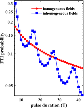
Figure 2. Probabilities of FTI as a function of laser pulse duration (specified by the number of cycles N) for the homogeneous (red circles) and inhomogeneous (blue squares) laser fields. The laser intensity is  W cm−2 and the laser wavelength is 800 nm.
Download figure:
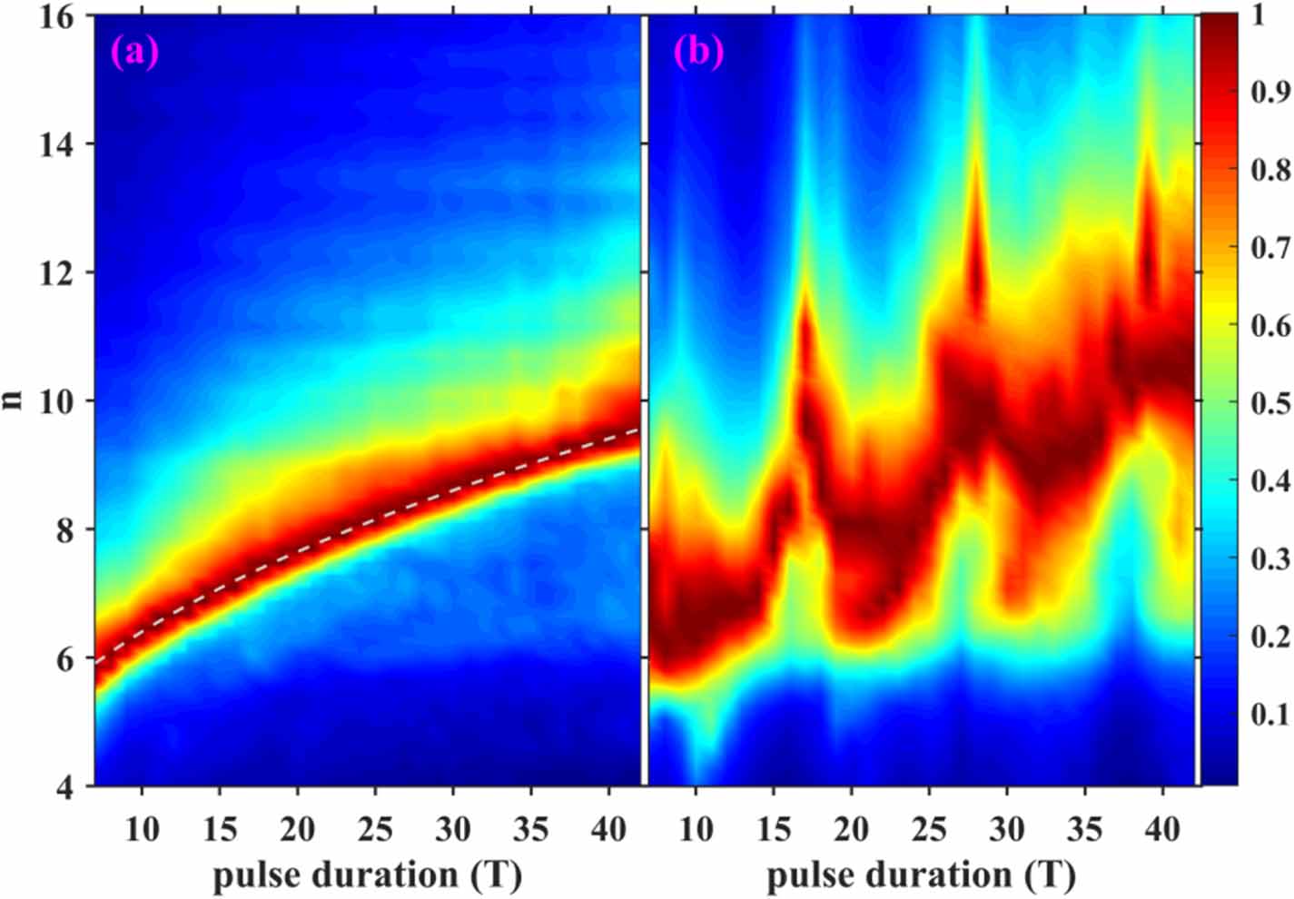
Standard image High-resolution imageIn figure 3, we present the principal quantum number n distributions for (a) homogeneous and (b) inhomogeneous laser fields as functions of pulse duration. In the case of homogeneous field, the dominant distribution of principal quantum number n increases with the increasing of laser pulse duration. The n increases gradually from 6 to 9 when the pulse duration number N is increased from 7 to 42. This is in excellent agreement with the theoretical prediction by the relation  (the dashed line) proposed in [19]. The underlying mechanism for this relation is that when the pulse duration exceeds a critical number of optical cycles, the pulled-out electrons can return to the ion core, resulting in elastic recollision and subsequent escape. Thus, an increasing in the pulse duration can deplete the lower-lying Rydberg states, and enhance the higher quantum number n [19]. However, the case of inhomogeneous field gives very different results, the dominant distribution of n shows a strong oscillatory structure, and has spikes at N = 17, 28 and 39, which are similar with the maxima of FTI probability curve in figure 2. Noteworthily, by replacing the trapezoidal pulse envelope
  in equation (3) with a more realistic cos2 envelope, we found that the FTI probability and the principal quantum number distribution as a function of the laser pulse duration still exhibit similar oscillatory behavior.

Figure 3. The principal quantum number distributions for (a) homogeneous and (b) inhomogeneous laser fields as a function of pulse duration in terms of optical cycles N, respectively. The white dashed line shows the prediction value  . The distribution is normalized individually with respect to the maximum at each T.
Download figure:
Standard image High-resolution imageTo understand the oscillations in the pulse duration dependence of the FTI probability and n-distribution driven by the inhomogeneous fields, we analyze the time evolution of the classical electron trajectories. For the sake of simplicity, we only analyze the trajectories with the tunneling occurs between  = 0.2 T and
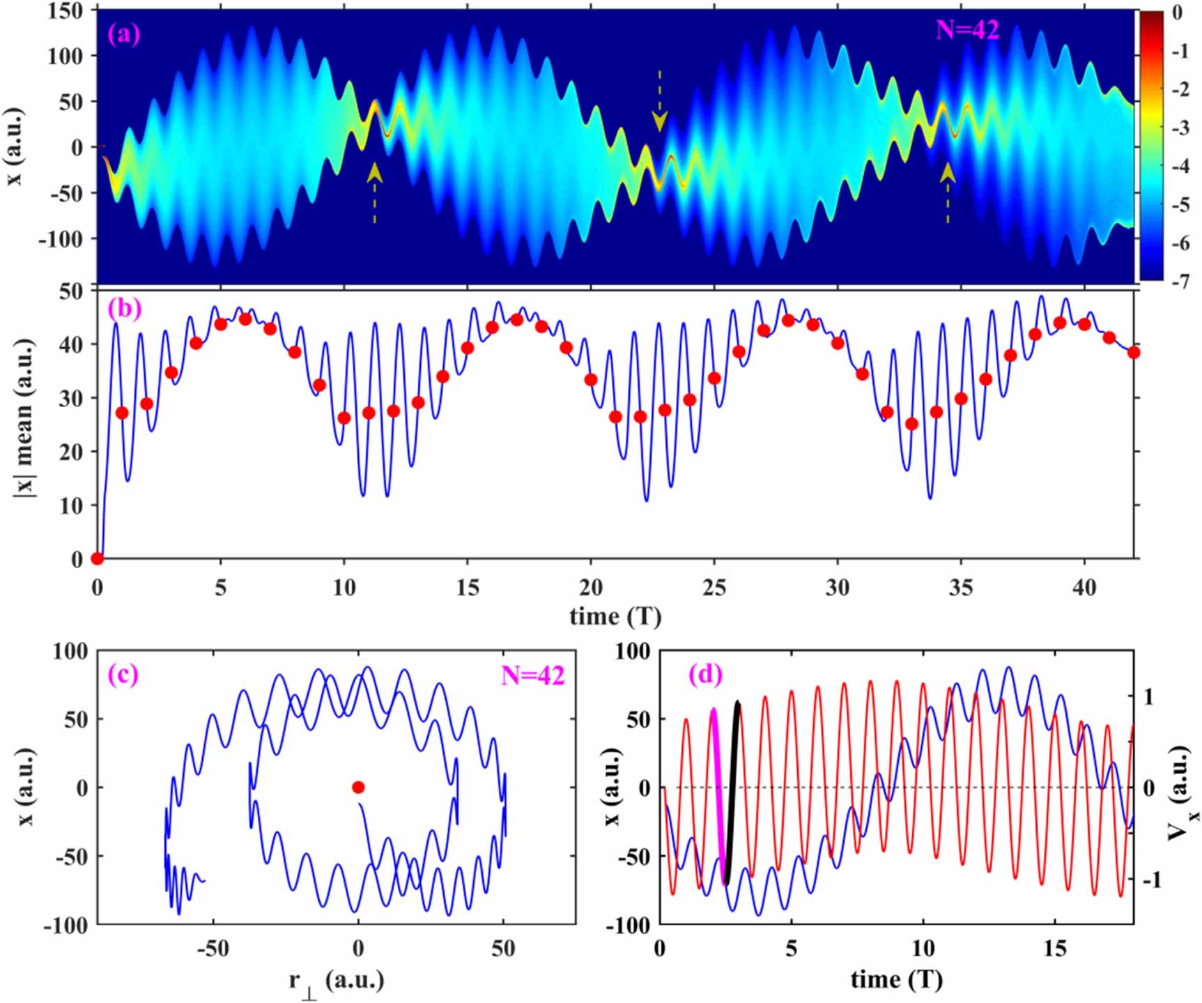
  = 0.3 T. It is justified to select only this tunneling time window due to the fact that the corresponding ADK ionization rate is 68% of the total ionization rate of the half of optical cycle, and FTI events occur centrally in this tunneling time window. Note that the results in figures 4 and 5 include all tunneling electrons, i.e. both the recaptured and ionized electrons. Figure 4(a) shows the time evolution of the tunneled electron's position distribution in the polarization direction of the field with pulse duration of 42 T. It is interesting that the spatial distribution of electron not only oscillating with period of the incident laser field, but also oscillating in a larger period of about 11 T, which is the same with the oscillating cycle of FTI yield and principal quantum number distribution in figures 2 and 3. When the electron is tunneling ionized from the atom, the electron defocusing occurs in the first few cycles, and then the spatial distribution is refocusing in the following 6th to 11th T. To help grasp the electron dynamic process more intuitively, figure 4(c) shows a sample FTI trajectory, and figure 4(d) shows the time evolution of the electron's position (red curve) and velocity (blue curve). Clearly, the electron's averaged position along the laser polarization direction is also oscillating in a large period. Taking 2 T to 3 T as an example, since the electron is far away from the parent ion at 2 T to 2.5 T, when the electric field reverses, the electron can experience a stronger electric field from 2.5 T to 3 T. The increase in velocity from 2.5 T to 3 T (solid black line in figure 4(d)) is larger than the decrease from 2 T to 2.5 T [solid pink line in figure 4(d)). Thus, as multiple optical cycles accumulate, the electron can return to the origin and oscillate in the gap of the nanostructure.

Figure 4. (a) The time evolution of the classical electron's position distribution in the polarization direction of the inhomogeneous fields for N = 42. Only the trajectories with the tunneling occurs between  = 0.2 T and
  = 0.3 T are analyzed. The distribution is normalized with respect to the maximum. (b) The mean value of the distance (in the polarization direction) from the ion core for the electron spatial distribution in (a). The red dots indicate the mean distance at the instants of integer optical cycles. (c) An example FTI trajectory. (d) The time evolution of the electron's position and velocity along the x-axis for the trajectory shown in (c), only the evolution during the first 18 T is shown.
Download figure:
Standard image High-resolution image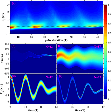
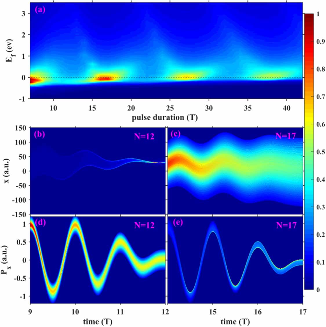
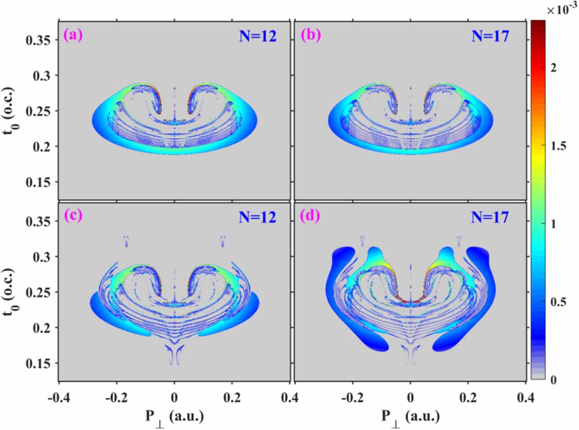
Figure 5. (a) Final energy distribution of all launched trajectories as a function of pulse duration (in number of optical cycles) for the inhomogeneous laser fields. (b)–(e) Spatial and momentum time evolution for N = 12 and 17, respectively. The FTI yield maximize (minimizes) for N = 17 (12), as shown in (a) and figure 2. Here, only the evolution during the last three optical cycles is shown. The distribution is normalized with respect to the maximum in each plot.
Download figure:
Standard image High-resolution imageOverall, the electron tunneling earlier can travel further away from the core in the inhomogeneous field, and thus experiences a stronger electric field. Then, it moves faster toward the origin when the direction of the electric field reverses. This results in the strong focusing of the electron spatial position distribution, as indicated by the arrows in figure 4(a). The strong focusing in the position space means a wide momentum distribution, and thus the position distribution spreads quickly again, resulting in the periodically defocusing and refocusing of the distribution, as shown in figure 4(a).
In figure 5(a), we present the final energy distribution of all launched trajectories as a function of pulse duration in terms of number of cycles for the inhomogeneous laser fields. It is obvious that the energy distribution has oscillation with the period of 11 T, similar to that in figure 4(a). For the pulse duration about 17 and 28 T, the dominant final energy is distributed around the 0 a.u. For the pulse duration about 12, 23 and 34 T, the final energy distribution spans over a larger region from negative to positive (up to about 2 a.u.). It means that more electrons can gain enough energy to escape from their parent ion, and thus less FTI events.
It is shown in figure 5(a) that the lower limit of final energy increases with pulse duration. Such trend is consistent with the increasing principal quantum number in figure 3. For the Rydberg electron, its quantum number n can be approximately estimated with  , where
  is the mean distance between the electron and the ion core [19, 22]. Figure 4(b) shows the time evolution of the mean distance with pulse duration of 42 T. One can see the mean distance of the ionized electron periodically oscillates with different amplitudes (the blue line). For the pulse duration with integer optical cycles (the red circles), the ionized electron acquires a sinusoidal oscillating mean distance, which gives rise to the oscillation structures in the n-distribution in figure 3(b).
To understand the physical picture above more intuitively, we present the last 3 T time evolution in spatial and momentum of electron trajectories with pulse duration of 12 T and 17 T in figures 5(b)–(e). For the case with pulse duration of 12 T, the spatial distribution of the electron is refocused near the origin at the end of the laser pulse, thus corresponding to the minimum peaks of the n-distribution oscillation (see figure 5(b)). For the case with pulse duration of 17 T, the spatial distribution of electron spreads out to the maximum, from −120 a.u. to 120 a.u., thus corresponding to the maximum position of the n-distribution oscillation (see figure 5(c)). As for the momentum distribution, as shown in figures 5(d) and (e), the final momentum is distributed in a large region of −0.3 to 0.3 a.u. for the pulse duration of 12 T. While for the case of 17 T, its final momentum distribution shrinks sharply, with the highest concentration around 0 a.u. Thus, the electron is more possible to be recaptured by the parent ion, resulting in high FTI yield, as shown in figure 2.
The oscillatory structures observed in the FTI probability curve (see figure 2) and the n-distribution (see figure 3(b)) are due to the above-mentioned repeating defocusing and refocusing. It is interesting to reveal how the oscillatory structure changes with the other laser field parameters.
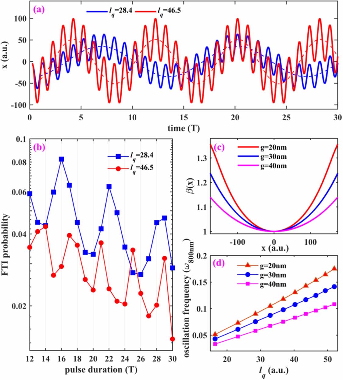
In the spatially inhomogeneous field, the electron propagation and acceleration can be characterized by the parameter  [29]. Figure 6(a) shows two classical trajectories released at
  = 0.25 T for
  = 28.4 (solid blue line) and
  = 46.5 (solid red line), respectively. Here, the
  can be adjusted by varying the intensity or the wavelength of the laser pulse. We can see that when
  increases, the oscillation periods of the guiding trajectories (dotted lines) decrease. It is 13 T for
  = 28.4 and 8 T for
  = 46.5. In figure 6(b), we present the probabilities of FTI as a function of pulse duration for
  = 28.4 and 46.5. One can see that the periods of oscillation structures are 6 T and 4 T respectively, which is in good agreement with half of the corresponding periods in figure 6(a). This significant dependence of the oscillation period on
  can be understood as follows. Increasing the
  causes the electron to travel farther from the parent ion in fewer optical cycle, thus experiencing a stronger laser field and returning to the parent ion faster when the electric field reverses. As a result, the period of the oscillating structure decreases rapidly.
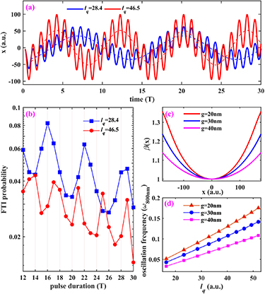
Figure 6. (a) The classical trajectories released at t0 = 0.25 T for lq
= 28.4 (blue line) and lq
= 46.5 (red line), respectively. (b) The probabilities of FTI as a function of laser pulse duration for lq
= 28.4 and 46.5. (c) The functional form of the inhomogeneity strength parameter  for
for  = 20, 30, 40 nm. (d) The oscillation frequency as a function of lq
for
= 20, 30, 40 nm. (d) The oscillation frequency as a function of lq
for  = 20 nm, 30 nm and 40 nm.
Download figure:
Standard image High-resolution imageThe FTI is also affected by the gap size g between the bow-tie nanostructure. The inhomogeneity strength parameter  with respect to the position inside the gap for
  = 20 nm, 30 nm and 40 nm are shown in figure 6(c). One can see that reducing the size of the gap between the bow-tie nanostructure can enhance the inhomogeneity strength. Then, we show the frequency of the oscillatory structure as a function of
  for the three different size of the gap, as depicted in figure 6(d). It can be seen that the oscillation frequency grows as the gap size reduces, since the stronger the laser field the electron feels as the electric field reverses, and the shorter the time for the electron to return to the parent ion, the higher the oscillation frequency. Thus, the amplitude of the electron quiver and the size of the gap between the bow-tie nanostructures are essential knobs for controlling the oscillatory structure.
3.2. The tunneling coordinates of FTI in the inhomogeneous fields
To reveal additional insight of the dynamics of the Rydberg electron driven by the inhomogeneous fields, we turn to the tunneling coordinates of the FTI events. We first examine the probability distributions of the FTI events in the coordinates of tunneling time  and initial transverse momentum
  for the homogeneous and the inhomogeneous fields for pulse durations where FTI yield achieves a minimum (N = 12) and maximum (N = 17). For the homogeneous fields, as shown in figures 7(a) and (b), the Rydberg electrons occupy crescent-shaped patches in both circumstances. The absence of the distributions with nearly zero initial transverse momentum is due to the rescattering process [19, 20]. In the inhomogeneous fields, as shown in figures 7(c) and (d), the electron tunneling ionized before the peak of the electric field with nearly zero initial transverse momentum is greatly suppressed, as compared to the homogeneous field. This is owing to the fact that the electron ionized within this area could be driven back to induce recollision in the inhomogeneous field.
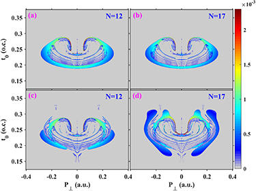
Figure 7. Probability distributions of the FTI events in the coordinates of the tunneling ionization time t0 and initial transverse momentum  for the homogeneous fields (top panels) and the inhomogeneous fields (bottom panels).
Download figure:
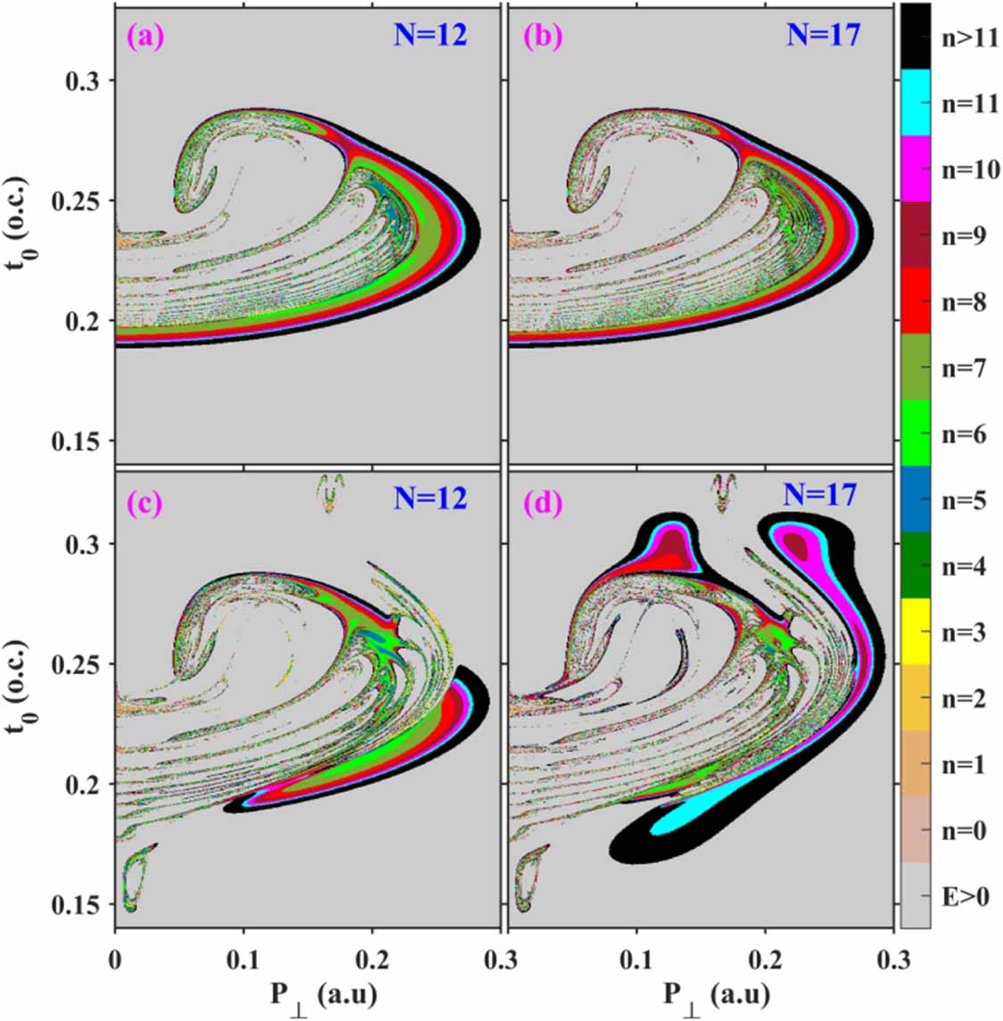
Standard image High-resolution imageMore details of the dynamic of the Rydberg electron can be found in the distributions of the principal quantum number n and the angular momentum L, which are important quantities for Rydberg atoms. In figure 8 we show the principal quantum number n in the coordinates of initial transverse momentum and tunneling time for different pulse durations in the homogeneous (top panels) and inhomogeneous (bottom panels) fields. For the homogeneous field, longer pulses preferentially deplete the low-lying Rydberg states, and thus the population in the inner side of the arc distribution is less for the longer pulse duration [19]. The distribution in the inhomogeneous field is very different from that of the homogeneous field. For the case of N = 17, the electron tunneling ionized far away from the peak of the electric field (0.25 T) can reach high principle number. This might be understood from the wide spread of the coordinate distribution in figure 5(c). For the case of N = 12, the area of the distribution shrinks significantly. It is worthwhile to mention that the periodic defocusing and refocusing of the electron spatial distribution can considerably increase the chance of rescattering, resulting in a faster fading of the FTI probability curve than that of homogeneous fields (see figure 2). Back tracing of the classical trajectories shows that the vanishing distribution around ( = 0.3 T,
  = 0.17 a.u.) in figure 8(d) results from the multiple re-scattering process.
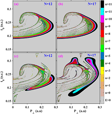
Figure 8. The distributions of principal quantum number n in the coordinates of the tunneling ionization time t0 and initial transverse momentum P⊥ for the homogeneous fields (a), (b) and the inhomogeneous fields (c), (d). (a), (c) for the N = 12, and (b), (d) for the N = 17. The colors represent the values of the principal quantum number n.
Download figure:
Standard image High-resolution imageFigure 9 displays the angular momentum L distributions in the initial transverse momentum and tunneling time coordinates for the N = 12 (left column) and 17 (right column) driven by the homogeneous (top panels) and inhomogeneous fields (bottom panels), respectively. For the homogeneous field, the maximum value of L is about 7, and the distribution stripes nearly parallel to the coordinate of tunneling time. However, in the inhomogeneous field, the angular momentum could reach much higher values, especially for the case of N = 17. The distribution of L shows a much more complicated behavior as compared to the case of the homogeneous field. This should be traced back to the complex electron dynamics of the tunneled electron in the inhomogeneous field, as shown in figure 4. These results indicate that the angular momentum of Rydberg electrons can be manipulated by changing the pulses duration of the inhomogeneous fields.

Figure 9. The distributions of angular momentum L in the coordinates of the tunneling ionization time t0 and initial transverse momentum P⊥ for the homogeneous fields (a), (b) and the inhomogeneous fields (c), (d). In (a), (c) the pulse duration is 12 T, and in (b), (d) the pulse duration is 17 T. The color represents the values of angular momentum L.
Download figure:
Standard image High-resolution image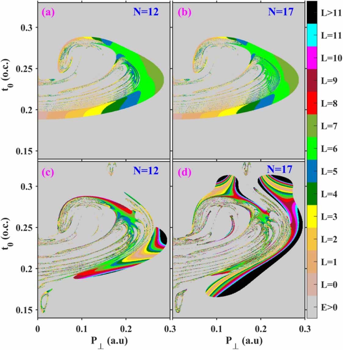
4. Conclusion
In summary, we explored the FTI driven by spatially inhomogeneous fields created by a bow-tie metal nanostructure using CTMC simulations. Our numerical results revealed the rhythmic oscillations of the FTI yield and the primary quantum number distribution as a function of the pulse duration. The frequency of this oscillation depends on the quiver amplitude of the tunneled electron in the inhomogeneous fields. By back-tracing the classical trajectories, we show that the oscillation structures originate from periodic defocusing and refocusing of the electron's spatial distribution. The pulse duration dependence of angular momentum distributions is also revealed. Our work suggests that the inhomogeneous field is an efficient tool to manipulate the dynamics of FTI in intense laser-atom interaction.
Acknowledgments
This work was supported by National Key Research and Development Program of China (Grants Nos. 2019YFA0308300, 2022YFE0134200); National Natural Science Foundation of China (Grants Nos. 11774131, 11874163, 12021004, 12074329, 1200432, 12104389 and 91850114); the Natural Science Foundation of Jilin Province, China (Grant No. 20220101016JC); Nanhu Scholars Program for Young Scholars of Xinyang Normal University; the Open Research Fund of State Key Laboratory of Transient Optics and Photonics. The computing work in this paper is supported by the Public Service Platform of High Performance Computing by Network and Computing Center of HUST.
Data availability statement
The data generated and/or analysed during the current study are not publicly available for legal/ethical reasons but are available from the corresponding author on reasonable request.