Probing the Purcell effect without radiative decay: lessons in the frequency and time domains

Ground-state fluctuations of the electromagnetic field in free space can be seen as responsible for observable effects such as the Lamb shift [1] or spontaneous emission [2]. Just as the ground-state fluctuations can alter states of matter, matter can in turn influence the quantum vacuum: ground-state fluctuations in close proximity to macroscopic objects—the so-called polaritonic or medium-assisted quantum vacuum—are inherently different from their free-space counterpart, see figure 1(b). Manipulating the quantum vacuum using optical environments, such as cavities or surface plasmon-polaritons, can thus be exploited to e.g. enhance or suppress spontaneous emission rates [3] or resonant energy transfer [4]. The environment-induced change of the Lamb shift leads to the Casimir–Polder force which acts on an atom in close proximity to a macroscopic object [5]. In the strong-coupling regime it even allows the alteration of chemical properties of molecules, for example their reaction rates [6, 7]. In the following, we will subsume all these environment-assisted quantum-vacuum effects under a generalised notion of the Purcell effect, which was originally conceived for the cavity-induced modification of spontaneous decay [3]. Besides its influence on atoms and molecules the changes of the quantum vacuum induced by macroscopic objects can also have an impact onto the macroscopic objects themselves; they lead e.g. to the Casimir force [8].

Zoom In Zoom Out Reset image size

A novel route to studying ground-state fluctuations of the electromagnetic field has been introduced by means of electro-optic sampling (EOS) experiments [9–11], see figure 1(a). In the setup described in reference [10] two linearly-polarised, ultra-short laser pulses propagate through a nonlinear crystal, in which they couple to vacuum fluctuations of the electromagnetic field via the nonlinear susceptibility inside the crystal. This coupling leads to a change of the polarisation direction of the laser pulses, which can be measured to infer information about the quantum vacuum inside the crystal on a sub-cycle time scale. This has been used to measure bare [9, 12] as well as squeezed [13, 14] quantum-vacuum noise. By tuning the temporal and spatial shifts between the two laser pulses, one can additionally detect vacuum correlations between distinct spatio-temporal regions and this way access the spectrum of the electromagnetic ground state [10], making EOS a promising tool for an in-depth study of medium-assisted vacuum fluctuations [15, 16].

In this work it is shown how EOS can be used to directly access environment-induced changes of the quantum vacuum. This is done for two examples. Firstly it is shown how the changes of the quantum vacuum induced by a perfectly reflecting plate or by a plate possessing a surface plasmon polariton can be revealed in the EOS signal. Secondly we discuss how the medium-assisted quantum vacuum inside a cavity consisting of the surfaces of the nonlinear crystal itself can be studied with unprecedented versatility. In all cases we assume parameters realizable in current experimental setups.

Furthermore, by interpreting ground-state correlations as the exchange of virtual photons (see also reference [17]), it is shown how one can observe the polaritonic quantum vacuum in the time domain. This e.g. allows one to study the dynamical formation of cavity modes in the quantum vacuum via multiple reflections, leading to a time-frequency uncertainty relation between the frequency resolution of the observed vacuum correlations and the time during which the quantum vacuum is observed.

To do so, we build upon previous theoretical results which have been introduced and compared to experimental data in references [15, 16] without consideration of the Purcell effect. The EOS signal accounting for absorption and dispersion inside the nonlinear crystal, as well as allowing for general optical environments and pump-pulse profiles, was found to be given by:

$$\begin{equation}g(\delta t,\delta {\mathbf{r}}_{{\Vert}})={\int }_{{V}_{\text{C}}} {\mathrm{d}}^{3}r {\int }_{{V}_{\text{C}}} {\mathrm{d}}^{3}{r}^{\prime } {\int }_{0}^{\infty }\mathrm{d}{\Omega}{\int }_{0}^{\infty }\mathrm{d}{{\Omega}}^{\prime }F(\mathbf{r},{\mathbf{r}}^{\prime },{\Omega},{{\Omega}}^{\prime },\delta {\mathbf{r}}_{{\Vert}},\delta t)\langle {\hat{E}}_{\text{vac},x}(\mathbf{r},{\Omega}){\hat{E}}_{\text{vac},x}^{{\dagger}}({\mathbf{r}}^{\prime },{{\Omega}}^{\prime })\rangle .\end{equation} \tag{ 1 }$$

Here, F(r, r', Ω, Ω', δ r_∥, δt) is a filter function depending on the spatio-temporal shape of the two laser pulses as well as on their lateral and temporal shifts δ r_∥ and δt, respectively, see appendix C, and V_C is the volume of the crystal. $\langle {\hat{\mathbf{E}}}_{\text{vac}}(\mathbf{r},{\Omega}){\hat{\mathbf{E}}}_{\text{vac}}^{{\dagger}}({\mathbf{r}}^{\prime },{{\Omega}}^{\prime })\rangle$ is the two-point ground-state correlation function of the electromagnetic field in an absorptive and dispersive optical environment, provided by macroscopic quantum electrodynamics as [18]

$$\begin{equation}\langle {\hat{\mathbf{E}}}_{\text{vac}}(\mathbf{r},{\Omega}){\hat{\mathbf{E}}}_{\text{vac}}^{{\dagger}}({\mathbf{r}}^{\prime },{{\Omega}}^{\prime })\rangle =\frac{\hslash {{\Omega}}^{2}}{{c}^{2}{\varepsilon }_{0}\pi }\delta ({\Omega}-{{\Omega}}^{\prime })\mathrm{I}\mathrm{m}\enspace \mathbf{G}(\mathbf{r},{\mathbf{r}}^{\prime },{\Omega}).\end{equation} \tag{ 2 }$$

Here, ɛ₀ is the free-space permittivity, c the speed of light in free space and $\mathbf{G}(\mathbf{r},{\mathbf{r}}^{\prime },{\Omega})$ is the dyadic Green's function describing the propagation of a photon at frequency Ω from r' to r, see appendix A. $\mathbf{G}$ and thus $\langle {\hat{\mathbf{E}}}_{\text{vac}}^{2}\rangle$ depend on the geometry of the optical environment (figure 1(b)). Note that the right-hand side of equation (2) can be connected to the local optical density of states by taking the trace as well as the coincidence limit of the Green's tensor [19]. Equation (1) suggests that by tuning the laser pulses and thus F, one can use EOS to access various characteristics of the two-point correlation functions of the electromagnetic ground state.

Throughout this paper we assume that all involved laser pulses are linearly polarised and Gaussian, with beam waist w = 80 μm, central frequency ω_c = 375 × 2π THz and pulse duration Δt = 80 fs, for details see appendix C. Unless stated otherwise, we consider the nonlinear crystal of length L = 0.1 mm to be a ZnTe crystal whose optical characteristics are summarized in appendix B.

In order to show how medium-induced changes of the quantum vacuum can be found in EOS experiments, we consider a plate and a cavity with different orientations, attached to the nonlinear crystal (see bottom right of figure 1(a)). In the presence of additional surfaces the Green's tensor splits into its bulk part ${\mathbf{G}}^{(0)}$ and scattering part ${\mathbf{G}}^{(1)}$ with $\mathbf{G}={\mathbf{G}}^{(0)}+{\mathbf{G}}^{(1)}$. The term ${\mathbf{G}}^{(1)}$ accounts for all reflection effects, such that restricting $\mathbf{G}$ to ${\mathbf{G}}^{(0)}$ is equivalent to neglecting all influences of any macroscopic object near to the nonlinear crystal as well as reflections at the surfaces of the crystal itself. We focus our attention on the changes these objects induce in the quantum vacuum correlations, and therefore neglect their influence on the laser pulses (aside from obscuring part of the beams). This can be justified by assuming that the reflection coefficients of the plate and the cavity are close to zero in the frequency range of the laser, but different from zero for the resolved frequencies of the vacuum field. Note, that this is a reasonable assumption—although the ultra-short laser pulses are broad in frequency space, the frequency range of the detected quantum vacuum (0–3) THz is well separated from that of the laser pulses (370–380) THz. Inserting the full Green's tensor into equation (1) we get two contributions, one stemming from the bulk ${\mathbf{G}}^{(0)}$ and one from the scattering part ${\mathbf{G}}^{(1)}$. The latter describes the change of the correlation function due to the presence of the macroscopic plate(s). Neglecting absorption effects inside the nonlinear crystal (e.g. ɛ(Ω) real-valued) and applying the 'laser paraxial' approximation suitable in the parameter range considered here [15, 16] the corresponding bulk (j = 0) and scattering (j = 1) contributions take the form

$$\begin{equation}{g}^{(j)}(\delta t,\delta {\mathbf{r}}_{{\Vert}})=C\underset{0{}}{\overset{\infty }{\int }}\mathrm{d}{\Omega}\enspace \mathrm{cos}({\Omega}\delta t){E}_{\text{vac}}^{2}({\Omega})\int \frac{{\mathrm{d}}^{2}{q}_{{\Vert}}}{4\pi {q}^{2}}{R}^{2}(\mathbf{q})\mathrm{R}\mathrm{e}[{p}^{(j)}(\mathbf{q},\delta {\mathbf{r}}_{{\Vert}}){O}^{(j)}(\mathbf{q},\delta {\mathbf{r}}_{{\Vert}})].\end{equation} \tag{ 3 }$$

For details of the derivation see appendix C. The full signal is given by g = g⁽⁰⁾ + g⁽¹⁾. In equation (3), $\sqrt{C}\propto {\chi }^{(2)}LI$ (L: length of the crystal, χ⁽²⁾: nonlinear susceptibility, I: intensity of the laser pulses) determines the sampling efficiency [10] and ${E}_{\text{vac}}^{2}({\Omega})$ gives the strength of the vacuum fluctuations in a bulk crystal at frequency Ω. The integral over the parallel wave vector of the vacuum field q_∥ ($q=n({\Omega}){\Omega}/c=\sqrt{{q}_{\perp }^{2}+{q}_{{\Vert}}^{2}}$) describes the propagation of the virtual photon from one laser pulse to the other. Here, O^(j)(q, δ r_∥) accounts for the obscuring of the beam due to the presence of the plate. Most importantly, this integral contains the propagation factor p^(j)(q, δ r_∥) which for the bulk contribution is simply given by ${p}^{(0)}={q}_{{\Vert}}^{2}/({q}_{\perp }q){\mathrm{e}}^{\text{i}\mathbf{q}\cdot \delta {\mathbf{r}}_{{\Vert}}}$, whereas p⁽¹⁾ depends on the chosen geometry of the attached plate(s). For a plate at x = −d for example one finds ${p}^{(1)}={p}^{(0)}{\mathrm{e}}^{2\text{i}{q}_{x}d}{R}_{p}$, where R_p is the p-polarised Fresnel reflection coefficient. The additional factor in p⁽¹⁾ compared to p⁽⁰⁾ accounts for the additional propagation of an exchanged virtual photon to the plate and back, see figure 3(a), and further discussion below. Similar expressions can be found for other geometries and a list of all propagation factors p⁽¹⁾ considered here is found in appendix C. Furthermore, the integral in equation (3) contains the known response function $R(\mathbf{q})={\mathrm{e}}^{-({q}_{x}^{2}+{q}_{y}^{2}){w}^{2}/8}\enspace \mathrm{s}\mathrm{i}\mathrm{n}\mathrm{c}\left\{L[{n}_{g}({\Omega}/c)-{q}_{z}]/2\right\}f({\Omega})$ [15, 16] accounting for the averaging over vacuum modes inside the finite lateral pulse profile, phase-matching and which contains the spectral autocorrelation function $f({\Omega})={\mathrm{e}}^{-\pi {{\Omega}}^{2}{\Delta}{t}^{2}/4}$.

We start by considering a reflecting plate attached to the nonlinear crystal in either the x = −d or y = −d planes, which is thus parallel to the propagation direction of the laser pulses offset by a distance d, see inset in the bottom right of figure 1(a). The contribution to the EOS signal with 'coincident' pulses (δt = δ r_∥ = 0) is shown in figure 2 as a function of d.

Zoom In Zoom Out Reset image size

First, in figure 2(a), we assume a perfectly reflecting plate described by reflection coefficients for p and s polarised waves R_p = 1 and R_s = −1, respectively. The EOS signal changes with the beam-plate distance as a result of competition between two effects. On the one hand, the signal decreases when the beam is closer to the plate, since a larger fraction of the beam becomes obscured by it. On the other hand, the effects of reflection upon the vacuum field start contributing significantly at a distance of approximately d = 4w. The opposite signs of these additional, plate-induced contributions ('scattering contributions') for the cases where the plate is in the x = −d or y = −d plane can be understood by realising that they arise from image fluctuations: in the former (latter) geometry the image-fluctuations are parallel (antiparallel) with respect to the x-polarised fluctuations of the quantum vacuum the laser pulse singles out. This leads to same (opposite) signs of the image fluctuating field compared to the bare fluctuations and thus to an enhancement (reduction) of the total fluctuating field. In both cases, the influence of the scattering contributions and thus of the plate-induced changes upon the quantum-vacuum correlations is clearly visible in the predicted full EOS signal.

A second model for the optical response of the plate is a Drude–Lorentz model permittivity defined by $\varepsilon ({\Omega})={\varepsilon }_{\infty }\left[1+{\omega }_{p}^{2}/({{\Omega}}^{2}-{\omega }_{\text{c}}^{2}+\text{i}{\Omega}{\Gamma})\right]$ with results shown in figure 2(b) for parameters ɛ_∞ = 8, ω_p = 0.86 × 2π THz, ω_c = 0.04 × 2π THz and Γ = 0.056 × 2π THz. These parameters are chosen such that the material's surface-plasmon polariton resonance coincides with the frequencies that the filter function picks out from the vacuum. Consequently there is a peak in the imaginary part of the Fresnel reflection coefficient R_p for p-polarized light as can be seen in the inset of figure 2(b), which corresponds to modes evanescent at the interface between the plate and the crystal. These evanescent modes dominate the spectrum of the vacuum's contribution to the variance and lead to an increase of the EOS signal by up to a factor of 5.5 when the beam gets close to the surface, cf figure 2(b).

We thus have revealed in which way one can use the EOS experiments to identify the changes of the medium-assisted quantum vacuum due to the coupling of the electromagnetic field to media. This makes EOS a suitable tool for in-depth study of the sculpted quantum vacuum in different optical environments. Revealing these environment-induced changes of the quantum vacuum would give one direct access to the physical origin of e.g. the Casimir or Casimir–Polder forces, the enhancement or reduction of spontaneous emission rates, or the Lamb shift in close proximity to macroscopic objects. As e.g. the spontaneous emission rate can be enhanced or reduced by perfectly reflecting plates or by surface plasmon polaritons, we can find a corresponding enhancement or reduction of the EOS signal.

Measuring these vacuum-induced effects is a formidable experimental task which usually only gives limited access to the structure of the quantum vacuum fluctuations—atoms and molecules are usually only sensitive to certain transition frequencies and the Casimir force results from an integration over all frequency space. In the following, we show how EOS can give a much more controlled and versatile access to medium-induced quantum vacuum fluctuations, especially in its ability to give a frequency and time domain perspective at the same time.

Thus far we have restricted the discussion to a frequency domain picture: the modes of the quantum-vacuum fluctuating at different frequencies are accessed by averaging them over the finite space-time volume of the laser pulses, cf equation (1). Revealing the microscopic processes involved leads to a complementary time-domain picture. As we discuss in more detail in appendix D, the basic mechanism leading to the EOS signal in equation (3) are two successive, nonlinear processes which are correlated via the quantum vacuum: in the first process a (virtual) photon is generated into the vacuum mode at position r [$\propto {\hat{E}}_{\text{vac},x}^{{\dagger}}(\mathbf{r})$] which is annihilated in a second process at position r' [$\propto {\hat{E}}_{\text{vac},x}({\mathbf{r}}^{\prime })$]. One example of two such correlated processes is displayed in figure 3(a) and is given by spontaneous parametric down-conversion and subsequent sum-frequency generation. The two photons which arise from this process are hence correlated and this correlation, which is proportional to the vacuum correlation function between the points r and r', is measured in EOS experiments of the quantum vacuum. On a microscopic level the observed process is hence an exchange of a virtual photon between two points within the nonlinear medium.

Zoom In Zoom Out Reset image size

The emerging time-domain picture of these experiments goes beyond their previous interpretation as a means to measure static, pre-existing vacuum-noise which can be squeezed or shaped by e.g. a cavity. Rather, the signal is interpreted as arising from the propagation of a virtual photon, which thus should experience retardation effects. To illustrate this, we study the signal as a function of the time delay between the pulses δt using different values for the beam separations δy, see figure 3(b). In figure 2(b) one sees that when δy becomes greater than the beam waist w we find maximal correlations for space-time regions which are shifted also in time by δyc_n as dictated by the finite velocity of the virtual photons. This is a clear signature of retardation effects in the quantum-vacuum correlations which also underlie all vacuum induced phenomena such as the Purcell effect and e.g. leads to the causal behaviour of Van der Waals forces between atoms mediated by such virtual photons [20, 21]. A direct observation of these effects in the EOS experiments discussed here would allow one to reveal these aspect of vacuum-induced phenomena.

In the virtual-photon picture of the quantum vacuum outlined in the last section, the changes of the quantum vacuum due to the presence of additional surfaces can be understood as follows: the virtual photon can not only propagate directly from r to r', but also propagate along a path which includes reflections from boundaries, see figure 3(a). The former (latter) is described by the bulk (scattering) Green's tensor ${\mathbf{G}}^{(0)}$ (${\mathbf{G}}^{(1)}$). Again, the dynamics of this process are not arbitrarily fast and, thus, in order to resolve it, the laser pulses which accesses the quantum vacuum must scan the quantum correlations for a time interval long enough such that (multiple) reflections can occur. This leads to a type of time-frequency uncertainty relation.

To show this dynamical aspect of the medium-induced quantum vacuum, we consider the effect of reflections from the front and back surfaces of the electro-optic crystal: these already constitute a planar cavity structure, see inset in the bottom right of figure 1(a). The electro-optic signal can be computed via equation (3) as before with O⁽⁰⁾ = O⁽¹⁾ = 1 and p^(j) given in appendix C. By definition, the bulk contribution remains unaffected by the surfaces, whereas for the scattering contribution the phase-matching condition in the response function selects only certain propagation paths. In order to be phase-matched, the virtual photon before and after reflection must propagate in the same direction as one of the two pulses such that it can be 'picked up' by that laser pulse. This means, for laser pulses propagating in the positive z-direction, only virtual photons which have been reflected at least twice can be phase-matched, see illustrations in figure 3(c).

The resulting signal as a function of δt is shown in the first row of figure 3(c). One finds that the scattering contribution is very small for δt = 0, since the pulses have already left the crystal (cavity) before the virtual photons have been reflected at least twice (this takes 2L/c_n = 2.1 ps, pulse duration Δt = 80 fs). This is again a clear signature of retardation effects in the vacuum correlation function. However, if the delay between the pulses δt is a multiple of 2L/c_n the second pulse arrives at the crystal precisely when the virtual photon generated by the first pulse has been reflected an even number of times. Thus the peaks for even values of δtc_n /L in figure 3(c) display its propagation in time domain. Fourier transforming the signal with respect to δt one can obtain the signal's spectrum g(Ω) [g(δt = 0) = ∫ dΩg(Ω)] [16], which shows the expected mode structure [see figure 1(b)] with resonances at multiples of c_n π/L, compare right-hand side of figure 3(c). However, in order to obtain g(Ω) experimentally one has to perform a measurement of g(δt) for a wide range of δt, i.e. one needs to resolve the correlations arising from different numbers of reflections individually in time. In the case of a single measurement at δt = 0, the positive and negative contributions in g⁽¹⁾(Ω) mostly cancel each other such that the cavity field remains unseen when it is averaged over a single space-time region. This can be seen as a time-frequency uncertainty relation.

To further improve the visibility of the cavity contribution we consider two beams propagating in opposite directions, i.e. the first into z, the second into −z. As a result, the bulk contribution is phase-mismatched and reduced considerably (see appendix C). The scattering contribution is dominated by that stemming from virtual photons which are reflected an odd number of times: they are generated by the first laser pulse propagating into z direction and are 'picked up' while propagating into −z direction by the second laser pulse. Since these virtual photons only have to propagate over a shorter distance compared to the configuration in which both pulses propagate into the same direction, this improves the visibility of the cavity modes, cf second row of figure 3(c).

Lastly, we consider the case where the durations of the laser pulses are much longer than the time a photon needs to propagate back and forth between the front and back side of the crystal, i.e. Δt ≫ L/c_n . In this case, multiple reflection can in principle occur but the spectral autocorrelation function restricts the accessed quantum vacuum to frequencies much shorter than the lowest resonant mode, i.e. f(Ω) = 0 for all Ω > c_n π/L. Hence, all the accessed modes interfere destructively so that in this case the vacuum field is completely suppressed such that g(0, 0) ≈ 0, compare lowest row of figure 3(c).

In this work we have shown how EOS can be exploited to measure environment-induced changes of the electromagnetic vacuum fluctuations (i.e. the Purcell effect) in the frequency and time domains. To do so, the signatures in the EOS signal resulting from the changes upon the quantum vacuum induced by a perfectly reflecting plate, by a surface plasmon polariton of an attached plate, or of a cavity have been calculated. It was shown, that in experimentally accessible parameter ranges EOS allows one to reveal and study these changes which lie at the heart of e.g. Casimir and Casimir–Polder forces, the Lamb shift or the enhancement of spontaneous emission rates of atoms in close proximity to macroscopic environments.

Interpreting vacuum correlations as arising from the exchange of virtual photons leads to a time domain picture of how vacuum correlations evolve which reveals retardation effects and a time-frequency uncertainty relation. For instance, the cavity-induced enhancement and suppression of vacuum fluctuations dynamically builds up via multiple reflections of such photons. We have shown how these dynamics of the (medium-assisted) quantum vacuum can be accessed in EOS experiments. This allows one to study dynamical aspects, such as retardation effects, of well established quantum-vacuum induced effects which can also be seen as arising from the exchange of virtual photons such as e.g. van der Waals forces, Casimir forces or resonant energy transfer. Vacuum fluctuations in the time domain also play a crucial role in the dynamical Casimir effect [22], where moving boundary conditions induce additional dynamics in the fluctuating vacuum field.

The time-domain picture of EOS given here, might also allow one to reveal how other space-time properties of the quantum-vacuum fluctuations can be accessed in EOS experiments in the future, such as vacuum correlations outside of the light-cone [23–26]. Future extensions might further include studying the vacuum field in more complex geometries such as plasmonic cavities [27].

The authors thank Jérôme Faist, Alexa Herter, Stephen Barnett, Denis Seletskiy, Guido Burkard and Alfred Leitenstorfer for fruitful discussions. RB acknowledges financial support by the Alexander von Humboldt Foundation, SYB thanks the Deutsche Forschungsgemeinschaft (Grant BU 1803/3-1476). FL acknowledges support from the Studienstiftung des deutschen Volkes. The article processing charge was funded by the Baden-Wuerttemberg Ministry of Science, Research and Art and the University of Freiburg in the funding programme Open Access Publishing.

No new data were created or analysed in this study.

The Green's tensor of the vector Helmholtz equation is defined via [18]

$$\begin{equation}\left(\nabla \times \nabla \times -\frac{{{\Omega}}^{2}}{{c}^{2}}\varepsilon (\mathbf{r},{\Omega})\right)\mathbf{G}(\mathbf{r},{\mathbf{r}}^{\prime },{\Omega})=\boldsymbol{\delta }(\mathbf{r}-{\mathbf{r}}^{\prime }),\end{equation} \tag{ A.1 }$$

with the boundary condition $\mathbf{G}(\mathbf{r},{\mathbf{r}}^{\prime },{\Omega})\to 0$ for |r − r'| → ∞. $\mathbf{G}$ can be subdivided into its bulk (${\mathbf{G}}^{(0)}$) and scattering (${\mathbf{G}}^{(1)}$) components such that $\mathbf{G}={\mathbf{G}}^{(0)}+{\mathbf{G}}^{(1)}$.

A.1. Bulk Green's tensor

The bulk Green's tensor solves equation (A.1) for an isotropic permittivity, i.e. ɛ(r, Ω) = ɛ(Ω). In a (2 + 1)-dimensional Weyl decomposition relative to a plane whose normal direction is denoted by r_⊥ it reads: [18]

$$\begin{align}{\mathbf{G}}^{(0)}(\mathbf{r},{\mathbf{r}}^{\prime },{\Omega})& =-\frac{1}{4{\pi }^{2}{k}^{2}(\omega )}\int {\mathrm{d}}^{2}{k}_{{\Vert}}\enspace \frac{{\mathrm{e}}^{\mathrm{i}{\mathbf{k}}_{{\Vert}}\cdot (\mathbf{r}-{\mathbf{r}}^{\prime })}}{{k}_{\perp }}\delta ({r}_{\perp }-{r}_{\perp }^{\prime }){\mathbf{e}}_{\perp }{\mathbf{e}}_{\perp }+\frac{i}{8{\pi }^{2}}\int {\mathrm{d}}^{2}{k}_{{\Vert}}\frac{{\mathrm{e}}^{\mathrm{i}{\mathbf{k}}_{{\Vert}}\cdot (\mathbf{r}-{\mathbf{r}}^{\prime })}}{{k}_{\perp }}\\\ & \quad \times \sum\limits _{\sigma =s,p} \left[{\mathbf{e}}_{\sigma +}{\mathbf{e}}_{\sigma +}{\mathrm{e}}^{\mathrm{i}{k}_{\perp }({r}_{\perp }-{r}_{\perp }^{\prime })}\theta ({r}_{\perp } -{r}_{\perp }^{\prime })\right.\\ & \quad +\left.{\mathbf{e}}_{\sigma -}{\mathbf{e}}_{\sigma -}{\mathrm{e}}^{-\mathrm{i}{k}_{\perp }({r}_{\perp }-{r}_{\perp }^{\prime })}\theta ({r}_{\perp }^{\prime } -{r}_{\perp })\right].\end{align} \tag{ A.2 }$$

Here, we have defined the wave vector $k=\sqrt{{\epsilon}({\Omega})}{\Omega}/c$, which can be split into perpendicular (k_⊥) and parallel (k_∥ = |k_∥|) components. Note that ${k}_{\perp }={k}_{\perp }({k}_{{\Vert}},{\Omega})=\sqrt{{k}^{2}-{k}_{{\Vert}}^{2}}$ with Im[k_⊥] > 0. The polarization vectors e_σ±, σ = s, p, are defined via

$$\begin{equation}{\mathbf{e}}_{s\pm }({\mathbf{k}}_{{\Vert}})={\mathbf{e}}_{{k}_{{\Vert}}}\times {\mathbf{e}}_{\perp },\end{equation} \tag{ A.3 }$$

$$\begin{equation}{\mathbf{e}}_{p\pm }({\mathbf{k}}_{{\Vert}})=\frac{1}{k}({k}_{{\Vert}}{\mathbf{e}}_{\perp }\mp {k}_{\perp }{\mathbf{e}}_{{k}_{{\Vert}}}).\end{equation} \tag{ A.4 }$$

A.2. Scattering Green's tensor

The scattering part of the Green's tensor depends on the geometry under consideration. Here, we are firstly interested in the geometry of a plate attached to the nonlinear crystal. Note, that we here neglect reflections from the surfaces of the crystal. We assume that the plate is thick enough such that it can be approximated by a semi-infinite half space with refractive index n'(Ω) whose interface is placed at r_⊥ < −d, with r_⊥ being the plate's normal vector. For the refractive index used to characterize the attached plate, see appendix B. For r_⊥ > −d we thus find the nonlinear crystal with refractive index n(Ω). In section 3 of the main text, we consider precisely this configuration with r_⊥ = x or r_⊥ = y. The scattering part of the Green's tensor inside the nonlinear crystal (${r}_{\perp },{r}_{\perp }^{\prime } > -d$) reads [18]

$$\begin{equation}{\mathbf{G}}^{(1)}(\mathbf{r},{\mathbf{r}}^{\prime },{\Omega})=\frac{i}{8{\pi }^{2}}\int {\mathrm{d}}^{2}{k}_{{\Vert}}\frac{{\mathrm{e}}^{\mathrm{i}{\mathbf{k}}_{{\Vert}}\cdot (\mathbf{r}-{\mathbf{r}}^{\prime })+\text{i}{k}_{\perp }({r}_{\perp }+{r}_{\perp }^{\prime }+2d)}}{{k}_{\perp }}\sum\limits _{\sigma =s,p}{R}_{\sigma }{\mathbf{e}}_{\sigma +}{\mathbf{e}}_{\sigma -}.\end{equation} \tag{ A.5 }$$

As in the main text, R_σ are the reflection coefficients at the nonlinear crystal/plate interface. In case of perfectly reflecting plates they are given by R_p = 1, R_s = −1 and in case of a plate with finite permittivity ' they are the usual Fresnel reflection coefficients which are given by

$$\begin{equation}{R}_{p}=\frac{{n}^{\prime }({\Omega}){k}_{\perp }-n({\Omega}){k}_{\perp }^{\prime }}{{n}^{\prime }({\Omega}){k}_{\perp }+n({\Omega}){k}_{\perp }^{\prime }},\end{equation} \tag{ A.6 }$$

$$\begin{equation}{R}_{s}=\frac{{k}_{\perp }-n({\Omega}){k}_{\perp }^{\prime }}{{k}_{\perp }+n({\Omega}){k}_{\perp }^{\prime }},\end{equation} \tag{ A.7 }$$

where ${k}_{\perp }^{\prime }=\sqrt{{n}^{\prime 2}({\Omega}){{\Omega}}^{2}/{c}^{2}-{q}_{{\Vert}}^{2}}$.

The other geometry considered in this work is that where reflections at the surfaces of the crystal are taken into account. This can be done by including the scattering part of the Green's tensor for a configuration where the refractive index for −L/2 < z < L/2 is given by the one of the nonlinear crystal and otherwise it is defined to be the vacuum refractive index, i.e. n'(Ω) = 1. For this geometry one finds [18]

$$\begin{align}{\mathbf{G}}^{(1)}(\mathbf{r},{\mathbf{r}}^{\prime },{\Omega})& =\frac{i}{8{\pi }^{2}}\int {\mathrm{d}}^{2}{k}_{{\Vert}}\frac{{\mathrm{e}}^{\mathrm{i}{\mathbf{k}}_{{\Vert}}\cdot (\mathbf{r}-{\mathbf{r}}^{\prime })}}{{k}_{\perp }}\sum\limits _{\sigma =s,p}\left\{\frac{{R}_{\sigma }{R}_{\sigma }{\mathrm{e}}^{2\text{i}{k}_{\perp }L}}{{D}_{\sigma }}\left[{\mathbf{e}}_{\sigma +}{\mathbf{e}}_{\sigma +}{\mathrm{e}}^{\text{i}{k}_{\perp }({r}_{\perp }-{r}_{\perp }^{\prime })}+{\mathbf{e}}_{\sigma -}{\mathbf{e}}_{\sigma -}{\mathrm{e}}^{-\text{i}{k}_{\perp }({r}_{\perp }-{r}_{\perp }^{\prime })}\right]\right.\\ & \quad \left.+\frac{1}{{D}_{\sigma }}\left[{\mathbf{e}}_{\sigma +}{\mathbf{e}}_{\sigma -}{R}_{\sigma }{\mathrm{e}}^{\text{i}{k}_{\perp }({r}_{\perp }+{r}_{\perp }^{\prime }+L)}+{\mathbf{e}}_{\sigma -}{\mathbf{e}}_{\sigma +}{R}_{\sigma }{\mathrm{e}}^{\text{i}{k}_{\perp }[L-{r}_{\perp }-{r}_{\perp }^{\prime }]}\right]\right\},\end{align} \tag{ A.8 }$$

for ${r}_{\perp },{r}_{\perp }^{\prime }\in [-L/2,L/2]$. Note that here we have chosen r_⊥ = z and ${k}_{\perp }={k}_{z}=\sqrt{k-{k}_{x}^{2}-{k}_{y}^{2}}$ and the terms ${D}_{\sigma }=1-{R}_{\sigma }{R}_{\sigma }{\mathrm{e}}^{2\text{i}{k}_{\perp }L}$ in the denominators account for multiple reflections. In the case that we assume that the crystal's surfaces are coated in order to increase the reflectivity in the THz range, we assume R_p = 0.95 and R_s = −0.95 and otherwise the reflection coefficients are given by equations (A.6) and (A.7) with n'(Ω) = 1.

In this section we give all optical parameters of the nonlinear crystal and its optical surroundings used in the main text to simulate the signal of EOS experiments.

The ordinary and group refractive indices of the nonlinear crystal at ω_c are n = 2.85 and n_g = 3.2 as measured in reference [28]. For the nonlinear refractive index we neglect its dispersion and use [28]

$$\begin{equation}{\chi }^{(2)}({\Omega})\approx {\chi }^{(2)}=\frac{{n}^{4}({\omega }_{\text{C}}){{\epsilon}}_{0}}{2}{r}_{41},\end{equation} \tag{ B.1 }$$

with r₄₁ = 1.17 × 10⁻²¹ CV⁻² [28].

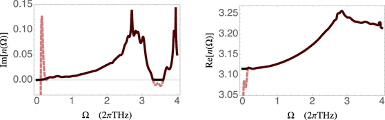
In the THz range we use the data for n which was measured using time domain spectroscopy in reference [10]. Its resulting real and imaginary part are shown in figure B1.

Zoom In Zoom Out Reset image size

For the plate attached to the nonlinear crystal which is described by a Drude–Lorentz model (figure 2(b) in the main text), we have used ${n}^{\prime }({\Omega})=\sqrt{{{\epsilon}}^{\prime }({\Omega})}$ with

$$\begin{equation}{{\epsilon}}^{\prime }({\Omega})={{\epsilon}}_{\infty }\left[1+\frac{{\omega }_{\text{p}}^{2}}{{{\Omega}}^{2}-{\omega }_{\text{c}}^{2}+\text{i}{\Omega}{\Gamma}}\right],\end{equation} \tag{ B.2 }$$

and _∞ = 8, ω_p = 0.86 × (2π) THz, ω_c = 0.04 × (2π) THz, Γ = 0.56 × (2π) THz.

In this section we derive analytic expressions for the electro-optic signal in the different geometries considered in the main text. The general approach is always the same and build upon equations (1) and (3) of the main text: one has to find the filter function as well as the Green's tensor for the different configurations, insert these expressions into equations (1) and (3) of the main text and solve as many of the resulting integrals as possible.

C.1. General equations

As shown in references [12, 15, 16], the electro-optic signal is given by

$$\begin{align}\hfill g& =\left\langle :\mathcal{S}\left\{\left(4\pi {{\epsilon}}_{0}c{\int }_{0}^{\infty }\mathrm{d}\omega \frac{\eta (\omega )}{\hslash \omega }\int {\mathrm{d}}^{2}{r}_{{\Vert}}\left[\text{i}{\hat{E}}_{1,y}^{{\dagger}}({\mathbf{r}}_{{\Vert}},\omega ){\hat{E}}_{1,x}({\mathbf{r}}_{{\Vert}},\omega )+\text{h.c.}\right]\right)\right.\right.\hfill \\ \hfill & \left.\left.\quad \times \left(4\pi {{\epsilon}}_{0}c{\int }_{0}^{\infty }\mathrm{d}\omega \frac{\eta (\omega )}{\hslash \omega }\int {\mathrm{d}}^{2}{r}_{{\Vert}}\left[\text{i}{\hat{E}}_{2,y}^{{\dagger}}({\mathbf{r}}_{{\Vert}},\omega ){\hat{E}}_{2,x}({\mathbf{r}}_{{\Vert}},\omega )+\text{h.c.}\right]\right)\right\}:\right\rangle .\hfill \end{align} \tag{ C.1 }$$

Here, η(ω) is the detector efficiency which is assumed to be one over the frequency range of the laser pulses, $\mathcal{S}$ is the symmetrization operator which is defined by its action onto a product of two operators ${\hat{O}}_{1,2}$: $\mathcal{S}{\hat{O}}_{1}{\hat{O}}_{2}=({\hat{O}}_{1}{\hat{O}}_{2}+{\hat{O}}_{2}{\hat{O}}_{1})/2$, :...: denotes normal ordering, ⟨...⟩ means that the ground state expectation value is taken, and ${\hat{\mathbf{E}}}_{1,2}$ is the electric field at detector 1 and 2, respectively. ${\hat{\mathbf{E}}}_{1,2}$ can be perturbatively expanded in terms of the nonlinear susceptibility χ⁽²⁾ and consists of the vacuum field ${\hat{\mathbf{E}}}_{\text{vac}}$, the classical probe field 1 (E_p,1) or 2 (E_p,2) and the field consisting of the nonlinear mixing of the vacuum field with either ${\mathbf{E}}_{p,1}$ or ${\mathbf{E}}_{p,2}$, respectively. This means, the electric field emerging from the crystal consists of the free fields (vacuum and coherent laser pulses) as well as of their mixing via the nonlinear coupling inside the crystal. See references [15, 16] for details. Allowing for absorption inside the crystal as well as general optical environments it was shown [15, 16] that g is given by equations (1) and (3) of the main text which are repeated here for clarity

$$\begin{equation}g(\delta t,\delta {\mathbf{r}}_{{\Vert}})={\int }_{{V}_{\text{C}}} {\mathrm{d}}^{3}r {\int }_{{V}_{\text{C}}} {\mathrm{d}}^{3}{r}^{\prime } {\int }_{0}^{\infty }\hspace{-8.5359pt}\mathrm{d}{\Omega}{\int }_{0}^{\infty }\hspace{-8.5359pt}\mathrm{d}{{\Omega}}^{\prime }F(\mathbf{r},{\mathbf{r}}^{\prime },{\Omega},{{\Omega}}^{\prime },\delta {\mathbf{r}}_{{\Vert}},\delta t)\langle {\hat{E}}_{\text{vac,}\;\text{x}}(\mathbf{r},{\Omega}){\hat{E}}_{\text{vac,}\;\text{x}}^{{\dagger}}({\mathbf{r}}^{\prime },{{\Omega}}^{\prime })\rangle ,\end{equation} \tag{ C.2 }$$

$$\begin{equation}\langle {\hat{\mathbf{E}}}_{\text{vac}}(\mathbf{r},{\Omega}){\hat{\mathbf{E}}}_{\text{vac}}^{{\dagger}}({\mathbf{r}}^{\prime },{{\Omega}}^{\prime })\rangle =\frac{\hslash {{\Omega}}^{2}}{{c}^{2}{\varepsilon }_{0}\pi }\delta ({\Omega}-{{\Omega}}^{\prime })\mathrm{I}\mathrm{m}\enspace \mathbf{G}(\mathbf{r},{\mathbf{r}}^{\prime },{\Omega}),\end{equation} \tag{ C.3 }$$

$$\begin{equation}\Longrightarrow(\delta t,\delta {\mathbf{r}}_{{\Vert}})=\frac{\hslash {{\Omega}}^{2}}{{c}^{2}{\varepsilon }_{0}\pi }{\int }_{{V}_{\text{C}}} {\mathrm{d}}^{3}r {\int }_{{V}_{\text{C}}} {\mathrm{d}}^{3}{r}^{\prime } {\int }_{0}^{\infty }\hspace{-8.5359pt}\mathrm{d}{\Omega}F(\mathbf{r},{\mathbf{r}}^{\prime },{\Omega},{{\Omega}}^{\prime },\delta {\mathbf{r}}_{{\Vert}},\delta t)\mathrm{I}\mathrm{m}\enspace \mathbf{G}(\mathbf{r},{\mathbf{r}}^{\prime },{\Omega}).\end{equation} \tag{ C.4 }$$

The filter function is given by

$$\begin{align}\hfill F(\mathbf{r},{\mathbf{r}}^{\prime },{\Omega},{{\Omega}}^{\prime })& =\frac{1}{2}\left\{\left[{H}_{1}(\mathbf{r},{\Omega})+{H}_{1}^{\ast }(\mathbf{r},-{\Omega})\right]\left[{H}_{2}({\mathbf{r}}^{\prime },-{{\Omega}}^{\prime })+{H}_{2}^{\ast }({\mathbf{r}}^{\prime },{{\Omega}}^{\prime })\right]\right.\hfill \\ \hfill & \left.\quad +\left[{H}_{2}(\mathbf{r},{\Omega})+{H}_{2}^{\ast }(\mathbf{r},-{\Omega})\right]\left[{H}_{1}({\mathbf{r}}^{\prime },-{{\Omega}}^{\prime })+{H}_{1}^{\ast }({\mathbf{r}}^{\prime },{{\Omega}}^{\prime })\right]\right\},\hfill \end{align} \tag{ C.5 }$$

with

$$\begin{equation}{H}_{i}({\mathbf{r}}^{\prime },{\Omega})=-8\pi \text{i}c{{\epsilon}}_{0}{\chi }^{(2)}({\Omega}){\mu }_{0}\underset{0{}}{\overset{\infty }{\int }}\mathrm{d}\omega \frac{\eta (\omega )\sqrt{{\epsilon}(\omega )}\omega }{\hslash }\int {\mathrm{d}}^{2}{r}_{{\Vert}}{E}_{p,i,y}^{\ast }({\mathbf{r}}_{{\Vert}},\omega ){\mathsf{G}}_{xx}({\mathbf{r}}_{{\Vert}},{\mathbf{r}}^{\prime },\omega ){E}_{p,i,y}({\mathbf{r}}^{\prime },\omega -{\Omega}).\end{equation} \tag{ C.6 }$$

To further simplify this expression, we insert the Gaussian laser pulse for E_p,i into equation (C.6), i.e. we use E_{p, i} (r, t) = ∫ dωE_{p, i} (r, ω)e^iωt with

$$\begin{equation}{\mathbf{E}}_{p,1}(\mathbf{r},\omega )={E}_{p}(\omega )\sqrt{\frac{2}{\pi {w}^{2}}}{\mathrm{e}}^{-{\mathbf{r}}_{{\Vert}}^{2}/{w}^{2}}{\mathrm{e}}^{\text{i}kz}{\mathbf{e}}_{y},\end{equation} \tag{ C.7 }$$

$$\begin{equation}{\mathbf{E}}_{p,2}(\mathbf{r},\omega )={E}_{p}(\omega )\sqrt{\frac{2}{\pi {w}^{2}}}{\mathrm{e}}^{-{({\mathbf{r}}_{{\Vert}}-\delta {\mathbf{r}}_{{\Vert}})}^{2}/{w}^{2}}{\mathrm{e}}^{\text{i}kz}{\mathrm{e}}^{\text{i}\omega \delta t}{\mathbf{e}}_{y},\end{equation} \tag{ C.8 }$$

$$\begin{equation}{E}_{p}(\omega )=\sqrt{\frac{{\Delta}t}{2}}{\mathrm{e}}^{-\pi {(\omega -{\omega }_{\text{c}})}^{2}{\Delta}{t}^{2}/2}.\end{equation} \tag{ C.9 }$$

Note, that here r_∥ = (x,y,0)^T , and k = n(ω)ω/c. Also we insert ${\mathsf{G}}_{xx}(\omega )={\mathsf{G}}_{xx}^{(0)}(\omega )$ with ${\mathbf{G}}^{(0)}$ given in equation (A.2) into equations (C.5) and (C.6). This is justified since throughout this work we assume that the optical environments do not affect the near-infrared laser pulses apart from obscuring them as discussed in the main text. Neglecting absorption in the frequency range of the laser pulses and applying the laser-paraxial approximation introduced in references [15, 16] one finds

$$\begin{align}\hfill F(\mathbf{r},{\mathbf{r}}^{\prime },{\Omega})& =2{\left(\frac{2{\chi }^{(2)}{\mu }_{0}cN{\omega }_{p}f({\Omega})}{{w}^{2}n({\omega }_{c})}\right)}^{2}{\mathrm{e}}^{-\text{i}{n}_{g}{\Omega}(z-{z}^{\prime })/c}\hfill \\ \hfill & \quad \times \left[{\mathrm{e}}^{-2\left[{\mathbf{r}}_{{\Vert}}^{2}+{({\mathbf{r}}_{{\Vert}}^{\prime }+\delta {\mathbf{r}}_{{\Vert}})}^{2}\right]/{w}^{2}}{\mathrm{e}}^{\text{i}{\Omega}\delta t}+{\mathrm{e}}^{-2\left[{\mathbf{r}}_{{\Vert}}^{\prime 2}+{({\mathbf{r}}_{{\Vert}}+\delta {\mathbf{r}}_{{\Vert}})}^{2}\right]/{w}^{2}}{\mathrm{e}}^{-\text{i}{\Omega}\delta t}\right].\hfill \end{align} \tag{ C.10 }$$

Here, n_g is the group refractive index at the central frequency ω_c of the laser pulse and ω_p and f(Ω) are the averaged detected frequency and the spectral autocorrelation function, respectively, given by

$$\begin{equation}{\omega }_{p}=\frac{{\int }_{0}^{\infty }\mathrm{d}\omega \eta (\omega ){E}_{p}^{2}(\omega )}{{\int }_{0}^{\infty }\mathrm{d}\omega \frac{\eta (\omega )}{\omega }{E}_{p}^{2}(\omega )},\end{equation} \tag{ C.11 }$$

$$\begin{equation}f({\Omega})=\frac{{\int }_{0}^{\infty }\mathrm{d}\omega \left[{E}_{p}(\omega ){E}_{p}(\omega +{\Omega})+{E}_{p}(\omega ){E}_{p}(\omega -{\Omega})\right]}{2{\int }_{0}^{\infty }\mathrm{d}\omega \eta (\omega ){E}_{p}{(\omega )}^{2}}\approx {\mathrm{e}}^{-\pi {{\Omega}}^{2}{\Delta}{t}^{2}/4}.\end{equation} \tag{ C.12 }$$

After having obtained the filter function, as well as the Green's tensor for the different geometries (see appendix A) we have all the ingredients needed in order to calculate the EOS signals in the different configurations using equations (1) and (C.3) which is done in the next two sections.

C.2. Plate with different orientations parallel to the propagation direction of the laser pulses

Here, we consider a plate which is parallel to the propagation direction of the laser pulses with two different orientations, i.e. in the x < −d and y < −d half spaces. We neglect absorption inside the nonlinear crystal by assuming (Ω) to be real. One can split the signal g in equation (C.4) into contributions stemming from the bulk and the scattering Green's tensors. Note, that although the bulk Green's tensor inside the nonlinear crystal is unaffected by the additional optical plates considered here, its contribution to the EOS signal still changes due to the fact that the laser pulses might get obscured by the plate whenever the pulse/plate distance becomes comparable to the beam waist. This is included in equation (C.4) by the restriction of the spatial integrals to the volume of the crystal V_C. These integrals become ${\int }_{{V}_{\text{C}}} {\mathrm{d}}^{3}r={\int }_{-L/2}^{L/2}\;\mathrm{d}z{\int }_{-\infty }^{\infty }\;\mathrm{d}y{\int }_{-d}^{\infty }\;\mathrm{d}x$ and ${\int }_{{V}_{\text{C}}} {\mathrm{d}}^{3}r={\int }_{-L/2}^{L/2}\;\mathrm{d}z{\int }_{-d}^{\infty }\;\mathrm{d}y{\int }_{-\infty }^{\infty }\;\mathrm{d}x$ for the two different orientations of the plate considered here, respectively. Inserting the bulk or scattering Green's tensors in equations (A.2) and (A.5) with r_⊥ chosen perpendicular to the applied surface and the filter function in equation (C.10) into equation (C.4) one finds after a tedious but straight forward calculation that the signal can always be brought into the form

$$\begin{equation}{g}^{(j)}(\delta t,\delta {\mathbf{r}}_{{\Vert}})=C\underset{0{}}{\overset{\infty }{\int }}\mathrm{d}{\Omega}\enspace \mathrm{cos}({\Omega}\delta t){E}_{\text{vac}}^{2}({\Omega})\int \frac{{\mathrm{d}}^{2}{q}_{{\Vert}}}{4\pi {q}^{2}}{R}^{2}(\mathbf{q})\mathrm{R}\mathrm{e}[{p}^{(j)}(\mathbf{q},\delta {\mathbf{r}}_{{\Vert}}){O}^{(j)}(\mathbf{q},\delta {\mathbf{r}}_{{\Vert}})].\end{equation} \tag{ C.13 }$$

This expression is identical to equation (3) of the main text. Here, $\sqrt{C}=2{\chi }^{(2)}L{\omega }_{\mathrm{p}}N(d,\delta {\mathbf{r}}_{{\Vert}})/n{{\epsilon}}_{0}c$ with N(d, δ r_∥) being the total number of detected photons given by

$$\begin{equation}{N}^{2}(d,\delta {\mathbf{r}}_{{\Vert}})=\frac{1}{4}\left(1+\mathrm{E}\mathrm{r}\mathrm{f}\left[\frac{\sqrt{2}d}{w}\right]\right)\left(1+\mathrm{E}\mathrm{r}\mathrm{f}\left[\frac{\sqrt{2}(d+\delta {\mathbf{r}}_{{\Vert}}\cdot \hat{\mathbf{n}})}{w}\right]\right){N}^{2},\end{equation} \tag{ C.14 }$$

$$\begin{equation}N=\frac{4\pi {{\epsilon}}_{0}cn({\omega }_{c})}{\hslash }{\int }_{0}^{\infty }\mathrm{d}\omega \frac{\eta (\omega )}{\omega }{E}_{p}^{2}(\omega ).\end{equation} \tag{ C.15 }$$

N is the total number of detected photons without the plate obscuring parts of the laser pulses, and $\mathrm{E}\mathrm{r}\mathrm{f}[x]=(2/\sqrt{\pi }){\int }_{0}^{x}\;\mathrm{d}t\enspace {\mathrm{e}}^{-{t}^{2}}$ is the error function. ${E}_{\text{vac}}^{2}({\Omega})$ is the coincidence limit of the bulk two-point correlation function of the electric field operator neglecting absorption effects and it reads

$$\begin{equation}{E}_{\text{vac}}^{2}({\Omega})=\frac{\hslash \enspace \mathrm{R}\mathrm{e}[n({\Omega})]{{\Omega}}^{3}}{2{{\epsilon}}_{0}{\pi }^{2}{c}^{3}}.\end{equation} \tag{ C.16 }$$

Also, note that the wave vector q has been split into a component which is parallel to the surface of the attached plate (q_∥) and one which is perpendicular to it (${q}_{\perp }=\sqrt{{q}^{2}-{q}_{{\Vert}}^{2}}$), with q = n(Ω)Ω/c. Finally, as also stated in the main text, the response function R(q) is given by

$$\begin{equation}{R}^{2}(\mathbf{q})={\mathrm{e}}^{-({q}_{x}^{2}+{q}_{y}^{2}){w}^{2}/4}\left\{{\mathrm{s}\mathrm{i}\mathrm{n}\mathrm{c}}^{2}\left[\frac{L}{2}\left({n}_{g}\frac{{\Omega}}{c}-{q}_{z}\right)\right]+{\mathrm{s}\mathrm{i}\mathrm{n}\mathrm{c}}^{2}\left[\frac{L}{2}\left({n}_{g}\frac{{\Omega}}{c}+{q}_{z}\right)\right]\right\}{f}^{2}({\Omega})\end{equation} \tag{ C.17 }$$

$$\begin{equation}\approx {\mathrm{e}}^{-({q}_{x}^{2}+{q}_{y}^{2}){w}^{2}/4}\enspace {\mathrm{s}\mathrm{i}\mathrm{n}\mathrm{c}}^{2}\left[\frac{L}{2}\left({n}_{g}\frac{{\Omega}}{c}-{q}_{z}\right)\right]{f}^{2}({\Omega}).\end{equation} \tag{ C.18 }$$

Here, we restricted the response in the second row to the phase-matched contribution only. Note, that this approximation is only a good approximation for propagating modes with q_∥ < Re[q]. It thus is used to calculate the EOS signal in figure 2(a) but not in figure 2(b), since in the latter case the main contribution to the scattering part of the signal stems from evanescent modes with q_∥ > Re[q].

The obscuring factors O^(j)(q, δ r_∥, d) in case of a plate in x < −d are given by

$$\begin{equation}{O}^{(0)}(\mathbf{q},\delta {\mathbf{r}}_{{\Vert}})=\frac{1}{4}\left(1+\mathrm{E}\mathrm{r}\mathrm{f}\left[\frac{\sqrt{2}d}{w}+\text{i}\frac{\text{i}{q}_{x}w}{2\sqrt{2}}\right]\right)\left(1+\mathrm{E}\mathrm{r}\mathrm{f}\left[\frac{\sqrt{2}(d+\delta x)}{w}-\text{i}\frac{\text{i}{q}_{x}w}{2\sqrt{2}}\right]\right),\end{equation} \tag{ C.19 }$$

$$\begin{equation}{O}^{(1)}(\mathbf{q},\delta {\mathbf{r}}_{{\Vert}})=\frac{1}{4}\left(1+\mathrm{E}\mathrm{r}\mathrm{f}\left[\frac{\sqrt{2}d}{w}+\text{i}\frac{\text{i}{q}_{x}w}{2\sqrt{2}}\right]\right)\left(1+\mathrm{E}\mathrm{r}\mathrm{f}\left[\frac{\sqrt{2}(d+\delta x)}{w}+\text{i}\frac{\text{i}{q}_{x}w}{2\sqrt{2}}\right]\right).\end{equation} \tag{ C.20 }$$

The expressions for O^(j)(q, δ r_∥) in case of a plate in y < −d can be obtained from equations (C.19) and (C.20) by replacing q_x ↔ q_y and δx ↔ δy.

Finally, the propagation factor p^(j) differs for the bulk and scattering contribution as well as for the different geometries (plates in x < −d or y < −d) and reads for the different configurations:

	Plate in x < −d, q⊥ = qx	Plate in y < −d, q⊥ = qy
p(0)(q, δ r∥)	$\frac{{q}_{{\Vert}}^{2}}{{q}_{\perp }q}{\mathrm{e}}^{\text{i}\delta {\mathbf{r}}_{{\Vert}}\cdot \mathbf{q}}$	$\frac{q}{{q}_{\perp }}\left(1-\frac{{q}_{{\Vert}}^{2}}{{q}^{2}}\right){\mathrm{e}}^{\text{i}\delta {\mathbf{r}}_{{\Vert}}\cdot \mathbf{q}}$
p(1)(q, δ r∥)	$\frac{{q}_{{\Vert}}^{2}}{{q}_{\perp }q}{\mathrm{e}}^{2\text{i}d{q}_{\perp }}{R}_{p}{\mathrm{e}}^{\text{i}\delta {\mathbf{r}}_{{\Vert}}\cdot \mathbf{q}}$	$\frac{q}{{q}_{\perp }}{\mathrm{e}}^{2\text{i}d{q}_{\perp }}\left({R}_{s}\frac{{q}_{z}^{2}}{{q}_{{\Vert}}^{2}}-{R}_{p}\frac{{q}_{\perp }^{2}{q}_{x}^{2}}{{q}_{{\Vert}}^{2}{q}^{2}}\right){\mathrm{e}}^{\text{i}\delta {\mathbf{r}}_{{\Vert}}\cdot \mathbf{q}}$.

C.3. Cavity setup: including reflections from the crystal's front and back surfaces

Similar to the last section, we can include the effect from reflections at the front and back surfaces of the crystal by using the appropriate scattering Green's tensor in addition to the bulk Green's tensor in equation (C.4). We first again neglect absorption by assuming that n(Ω) is real. The bulk contribution is not further restricted in this configuration and thus agrees with the signal considered in previous studies in which reflection effects have been neglected [15, 16]. It can be derived by using the bulk Green's tensor (equation (A.2)) in equation (C.4) and the resulting expression is again given by equation (3) with q_⊥ = q_z , O^(j)(q, δ r_∥) = 1, N(d, δ r_∥) = N and ${p}^{(0)}(\mathbf{q},\delta {\mathbf{r}}_{{\Vert}})=q\frac{1-{q}_{x}^{2}/{q}^{2}}{2{q}_{\perp }}{\mathrm{e}}^{\text{i}\mathbf{q}\cdot \delta {\mathbf{r}}_{{\Vert}}}$. The scattering contribution is obtained by inserting the Green's tensor of the cavity in equation (A.8) into equation (C.4). After some calculation very similar to the ones in the last section one obtains

$$\begin{align}{g}^{(1)}(\delta t,\delta {\mathbf{r}}_{{\Vert}})& =C\underset{0{}}{\overset{\infty }{\int }}\mathrm{d}{\Omega}\enspace \mathrm{cos}({\Omega}\delta t){E}_{\text{vac}}^{2}({\Omega}){f}^{2}({\Omega})\int \frac{{\mathrm{d}}^{2}{q}_{{\Vert}}}{4\pi {q}^{2}}{\mathrm{e}}^{-({q}_{x}^{2}+{q}_{y}^{2}){w}^{2}/4}\\\ & \quad \times \mathrm{R}\mathrm{e}\left\{\frac{q}{{q}_{\perp }}{\mathrm{e}}^{\text{i}\mathbf{q}\cdot \delta {\mathbf{r}}_{{\Vert}}}{\mathrm{e}}^{2\text{i}{q}_{\perp }L}\left(\frac{{R}_{s}^{2}{q}_{y}^{2}}{{D}_{s}{q}_{{\Vert}}^{2}}+\frac{{R}_{p}^{2}{q}_{x}^{2}{q}_{\perp }^{2}}{{D}_{p}{q}^{2}{q}_{{\Vert}}^{2}}\right)\right.\\\ & \quad \times \left.\left(\mathrm{s}\mathrm{i}\mathrm{n}{\mathrm{c}}^{2}\left[\frac{L}{2}\left({n}_{g}\frac{{\Omega}}{c}-{q}_{z}\right)\right]+\mathrm{s}\mathrm{i}\mathrm{n}{\mathrm{c}}^{2}\left[\frac{L}{2}\left({n}_{g}\frac{{\Omega}}{c}+{q}_{z}\right)\right]\right)\right.\\ & \quad \left.+\frac{2q}{{q}_{\perp }}{\mathrm{e}}^{\text{i}\mathbf{q}\cdot \delta {\mathbf{r}}_{{\Vert}}}{\mathrm{e}}^{\text{i}{q}_{\perp }L}\left(\frac{{R}_{s}{q}_{y}^{2}}{{D}_{s}{q}_{{\Vert}}^{2}}-\frac{{R}_{p}{q}_{x}^{2}{q}_{\perp }^{2}}{{D}_{p}{q}^{2}{q}_{{\Vert}}^{2}}\right)\mathrm{s}\mathrm{i}\mathrm{n}\mathrm{c}\left[\frac{L}{2}\left({n}_{g}\frac{{\Omega}}{c}-{q}_{z}\right)\right]\mathrm{s}\mathrm{i}\mathrm{n}\mathrm{c}\left[\frac{L}{2}\left({n}_{g}\frac{{\Omega}}{c}+{q}_{z}\right)\right]\right\}.\end{align} \tag{ C.21 }$$

In the case that the crystal length is very short, e.g. set to L = 1 μm (third row of figure 3(c) in the main plot), one needs to take all these terms into account. However, in case L = 0.1 mm (as used throughout the rest of the paper) it is enough to only include the phase-matched contribution, i.e. only the term proportional to ${\mathrm{s}\mathrm{i}\mathrm{n}\mathrm{c}}^{2}\left[L\left({n}_{g}({\Omega}/c)-{q}_{z}\right)/2\right]$. In this case we can again bring equation (C.21) into the form of equation (3) with q_⊥ = q_z , O(q, δ r_∥, d) = 1, N(d, δ r_∥) = N, the response function given by equation (C.18) and

$$\begin{equation}{p}^{(1)}(\mathbf{q},\delta {\mathbf{r}}_{{\Vert}})=\frac{q}{{q}_{\perp }}{\mathrm{e}}^{\text{i}\mathbf{q}\cdot \delta {\mathbf{r}}_{{\Vert}}}{\mathrm{e}}^{2\text{i}{q}_{\perp }L}\left(\frac{{R}_{s}^{2}{q}_{y}^{2}}{{D}_{s}{q}_{{\Vert}}^{2}}+\frac{{R}_{p}^{2}{q}_{x}^{2}{q}_{\perp }^{2}}{{D}_{p}{q}^{2}{q}_{{\Vert}}^{2}}\right).\end{equation} \tag{ C.22 }$$

Note, that this propagation factor only includes contributions which are at least quadratic in the reflection coefficients, meaning that the virtual photon is reflected at least twice.

In the case where the two pulses are assumed to propagate in opposite direction one has to replace e^ikz by e^−ikz in equation (C.8). The calculation is very similar to the one before. For the bulk contribution, the result is again given by equation (3) with q_⊥ = q_z , O(q, δ r_∥, d) = 1, N(d, δ r_∥) = N and ${p}^{(0)}=q\frac{1-{q}_{x}^{2}/{q}^{2}}{{q}_{\perp }}{\mathrm{e}}^{\text{i}\mathbf{q}\cdot \delta {\mathbf{r}}_{{\Vert}}}$ as for the case were the two pulses propagate into the same direction but the response function now reads

$$\begin{equation}{R}^{2}(\mathbf{q})={\mathrm{e}}^{-({q}_{x}^{2}+{q}_{y}^{2}){w}^{2}/4}\enspace \mathrm{s}\mathrm{i}\mathrm{n}\mathrm{c}\left[\frac{L}{2}\left({n}_{g}\frac{{\Omega}}{c}-{q}_{z}\right)\right]\mathrm{s}\mathrm{i}\mathrm{n}\mathrm{c}\left[\frac{L}{2}\left({n}_{g}\frac{{\Omega}}{c}+{q}_{z}\right)\right]f({\Omega}).\end{equation} \tag{ C.23 }$$

We see that there is no phase-matched contribution as expected since the two pulses propagate into opposite directions. The scattering contribution is also given by equation (3) with q_⊥ = q_z , O(q, δ r_∥, d) = 1, N(d, δ r_∥) = N, the response function in equation (C.18) and

$$\begin{equation}{p}^{(1)}(\mathbf{q},\delta {\mathbf{r}}_{{\Vert}})=\frac{q}{{q}_{\perp }}{\mathrm{e}}^{\text{i}\mathbf{q}\cdot \delta {\mathbf{r}}_{{\Vert}}}{\mathrm{e}}^{\text{i}{q}_{\perp }L}\left(\frac{{R}_{s}{q}_{y}^{2}}{{D}_{s}{q}_{{\Vert}}^{2}}-\frac{{R}_{p}{q}_{x}^{2}{q}_{\perp }^{2}}{{D}_{p}{q}^{2}{q}_{{\Vert}}^{2}}\right).\end{equation} \tag{ C.24 }$$

Note, that this propagation factor now includes contribution which are proportional to R_σ , meaning that the virtual photon can this time also be reflected only once and still be phase-matched as expected.

Lastly, we calculate the signal accounting not only for reflections at the front and back surfaces of the crystal but also for absorption in the THz region. To do so we allow n(Ω) to have a nonvanishing imaginary part (compare right-hand side of figure B1). For the bulk contribution with both pulses propagating into the same direction one finds as previously also obtained in reference [15]

$$\begin{align}\hfill {g}^{(0)}(\delta t,\delta {\mathbf{r}}_{{\Vert}})& =C\underset{0{}}{\overset{\infty }{\int }}\mathrm{d}{\Omega}\enspace \mathrm{cos}({\Omega}\delta t){E}_{\text{vac}}^{2}({\Omega}){f}^{2}({\Omega})\int \frac{{\mathrm{d}}^{2}{q}_{{\Vert}}}{4\pi \mathrm{R}\mathrm{e}[q]}{\mathrm{e}}^{-({q}_{x}^{2}+{q}_{y}^{2}){w}^{2}/4}\hfill \\ \hfill & \quad \times \mathrm{R}\mathrm{e}\left[{\mathrm{e}}^{\text{i}\mathbf{q}\cdot \delta {\mathbf{r}}_{{\Vert}}}\frac{\left(1-\frac{{q}_{x}^{2}}{{q}^{2}}\right)}{{q}_{z}{L}^{2}}\left(\frac{\text{i}L}{{q}_{z}-{n}_{g}{\Omega}/c}+\frac{1-{\mathrm{e}}^{\text{i}L({q}_{z}-{n}_{g}{\Omega}/c)}}{{({q}_{z}-{n}_{g}{\Omega}/c)}^{2}}\right)\right].\hfill \end{align} \tag{ C.25 }$$

Here, only the phase-matched contribution is included.

For the scattering contribution we repeat the same calculation leading to equation (C.21) but allowing for an imaginary part of n(Ω). This leads to

$$\begin{align}\hfill {g}^{(1)}(\delta t,\delta {\mathbf{r}}_{{\Vert}})& =C\underset{0{}}{\overset{\infty }{\int }}\mathrm{d}{\Omega}\enspace \mathrm{cos}({\Omega}\delta t){E}_{\text{vac}}^{2}({\Omega}){f}^{2}({\Omega})\int \frac{{\mathrm{d}}^{2}{q}_{{\Vert}}}{4\pi \mathrm{R}\mathrm{e}[q]}{\mathrm{e}}^{-({q}_{x}^{2}+{q}_{y}^{2}){w}^{2}/4}\hfill \\ \hfill & \quad \times \mathrm{R}\mathrm{e}\left\{\frac{1}{{q}_{\perp }}{\mathrm{e}}^{\text{i}\mathbf{q}\cdot \delta {\mathbf{r}}_{{\Vert}}}{\mathrm{e}}^{2\text{i}{q}_{\perp }L}\left(\frac{{R}_{s}^{2}{q}_{y}^{2}}{{D}_{s}{q}_{{\Vert}}^{2}}+\frac{{R}_{p}^{2}{q}_{x}^{2}{q}_{\perp }^{2}}{{D}_{p}{q}^{2}{q}_{{\Vert}}^{2}}\right)\right.\hfill \\ \hfill & \quad \times \left.\left({\mathrm{s}\mathrm{i}\mathrm{n}\mathrm{c}}^{2}\left[\frac{L}{2}\left({n}_{g}\frac{{\Omega}}{c}-{q}_{z}\right)\right]+{\mathrm{s}\mathrm{i}\mathrm{n}\mathrm{c}}^{2}\left[\frac{L}{2}\left({n}_{g}\frac{{\Omega}}{c}+{q}_{z}\right)\right]\right)\right.\hfill \\ \hfill & \quad \left.+\frac{2}{{q}_{\perp }}{\mathrm{e}}^{\text{i}\mathbf{q}\cdot \delta {\mathbf{r}}_{{\Vert}}}{\mathrm{e}}^{\text{i}{q}_{\perp }L}\left(\frac{{R}_{s}{q}_{y}^{2}}{{D}_{s}{q}_{{\Vert}}^{2}}-\frac{{R}_{p}{q}_{x}^{2}{q}_{\perp }^{2}}{{D}_{p}{q}^{2}{q}_{{\Vert}}^{2}}\right)\mathrm{s}\mathrm{i}\mathrm{n}\mathrm{c}\left[\frac{L}{2}\left({n}_{g}\frac{{\Omega}}{c}-{q}_{z}\right)\right]\mathrm{s}\mathrm{i}\mathrm{n}\mathrm{c}\left[\frac{L}{2}\left({n}_{g}\frac{{\Omega}}{c}+{q}_{z}\right)\right]\right\}.\hfill \end{align} \tag{ C.26 }$$

In the case where the two pulses propagate into opposite direction and absorption effects are considered, the bulk contribution to the signal is given by

$$\begin{align}\hfill {g}^{(0)}(\delta t,\delta {\mathbf{r}}_{{\Vert}})& =C\underset{0{}}{\overset{\infty }{\int }}\mathrm{d}{\Omega}\enspace \mathrm{cos}({\Omega}\delta t){E}_{\text{vac}}^{2}({\Omega}){f}^{2}({\Omega})\int \frac{{\mathrm{d}}^{2}{q}_{{\Vert}}}{4\pi \mathrm{R}\mathrm{e}[q]}{\mathrm{e}}^{-({q}_{x}^{2}+{q}_{y}^{2}){w}^{2}/4}\hfill \\ \hfill & \quad \times \mathrm{R}\mathrm{e}\left[{\mathrm{e}}^{\text{i}\mathbf{q}\cdot \delta {\mathbf{r}}_{{\Vert}}}\frac{\left(1-\frac{{q}_{x}^{2}}{{q}^{2}}\right)}{{q}_{z}{L}^{2}}\left(\frac{\text{i}\frac{{q}_{z}c}{{n}_{g}{\Omega}}\enspace \mathrm{sin}(L{n}_{g}{\Omega}/c)+\mathrm{cos}(L{n}_{g}{\Omega}/c)-{\mathrm{e}}^{\text{i}L{q}_{z}}}{({q}_{z}-{n}_{g}{\Omega}/c)({q}_{z}+{n}_{g}{\Omega}/c)}\right)\right].\hfill \end{align} \tag{ C.27 }$$

and the scattering contribution by

$$\begin{align}\hfill {g}^{(1)}(\delta t,\delta {\mathbf{r}}_{{\Vert}})& =C\underset{0{}}{\overset{\infty }{\int }}\mathrm{d}{\Omega}\enspace \mathrm{cos}({\Omega}\delta t){E}_{\text{vac}}^{2}({\Omega}){f}^{2}({\Omega})\int \frac{{\mathrm{d}}^{2}{q}_{{\Vert}}}{4\pi \mathrm{R}\mathrm{e}[q]}{\mathrm{e}}^{-({q}_{x}^{2}+{q}_{y}^{2}){w}^{2}/4}\hfill \\ \hfill & \quad \times \mathrm{R}\mathrm{e}\left\{\frac{2}{{q}_{\perp }}{\mathrm{e}}^{\text{i}\mathbf{q}\cdot \delta {\mathbf{r}}_{{\Vert}}}{\mathrm{e}}^{2\text{i}{q}_{\perp }L}\left(\frac{{R}_{s}^{2}{q}_{y}^{2}}{{D}_{s}{q}_{{\Vert}}^{2}}+\frac{{R}_{p}^{2}{q}_{x}^{2}{q}_{\perp }^{2}}{{D}_{p}{q}^{2}{q}_{{\Vert}}^{2}}\right)\mathrm{s}\mathrm{i}\mathrm{n}\mathrm{c}\left[\frac{L}{2}\left({n}_{g}\frac{{\Omega}}{c}-{q}_{z}\right)\right]\mathrm{s}\mathrm{i}\mathrm{n}\mathrm{c}\left[\frac{L}{2}\left({n}_{g}\frac{{\Omega}}{c}+{q}_{z}\right)\right]\right.\hfill \\ \hfill & \quad \left.+\frac{1}{{q}_{\perp }}{\mathrm{e}}^{\text{i}\mathbf{q}\cdot \delta {\mathbf{r}}_{{\Vert}}}{\mathrm{e}}^{\text{i}{q}_{\perp }L}\left(\frac{{R}_{s}{q}_{y}^{2}}{{D}_{s}{q}_{{\Vert}}^{2}}-\frac{{R}_{p}{q}_{x}^{2}{q}_{\perp }^{2}}{{D}_{p}{q}^{2}{q}_{{\Vert}}^{2}}\right)\right.\hfill \\ \hfill & \quad \times \left.\left({\mathrm{s}\mathrm{i}\mathrm{n}\mathrm{c}}^{2}\left[\frac{L}{2}\left({n}_{g}\frac{{\Omega}}{c}-{q}_{z}\right)\right]+{\mathrm{s}\mathrm{i}\mathrm{n}\mathrm{c}}^{2}\left[\frac{L}{2}\left({n}_{g}\frac{{\Omega}}{c}+{q}_{z}\right)\right]\right)\right\}.\hfill \end{align} \tag{ C.28 }$$

We discuss the microscopic processes leading to the contribution to the signal's variance found in equation (1). We first realize that, on the one hand, terms of the structure ${\hat{E}}_{x}({\mathbf{r}}^{\prime },{\Omega}){\hat{E}}_{y}({\mathbf{r}}^{\prime },\omega -{\Omega}){G}_{xx}(\mathbf{r},{\mathbf{r}}^{\prime },\omega )$ correspond to a processes generally referred to as sum-frequency generation [29]. Here an atom absorbs two photons with polarization x, y and frequency Ω, ω − Ω respectively and the excited atom subsequently emits an x polarized photon with frequency ω. On the other hand, terms of the structure ${\hat{E}}_{x}^{{\dagger}}({\mathbf{r}}^{\prime },{\Omega}){\hat{E}}_{y}({\mathbf{r}}^{\prime },\omega +{\Omega}){G}_{xx}(\mathbf{r},{\mathbf{r}}^{\prime },\omega )$ describe the process of parametric down-conversion [29], where an atom is excited by one photon of frequency ω + Ω which subsequently deexcites by a two-photon emission process where both photons are x-polarised and have frequencies Ω and ω, respectively.Now let us turn our attention to equation (C.1), i.e.

$$\begin{align}\hfill g& =\mathcal{S}\left\{\left(4\pi {{\epsilon}}_{0}c{\int }_{0}^{\infty }\mathrm{d}\omega \frac{\eta (\omega )}{\hslash \omega }\int {\mathrm{d}}^{2}{r}_{{\Vert}}\left[\text{i}{\hat{E}}_{y,1}^{{\dagger}}({\mathbf{r}}_{{\Vert}},\omega ){\hat{E}}_{x,1}({\mathbf{r}}_{{\Vert}},\omega )+\text{h.c.}\right]\right)\right.\hfill \\ \hfill & \quad \left.\times \left(4\pi {{\epsilon}}_{0}c{\int }_{0}^{\infty }\mathrm{d}\omega \frac{\eta (\omega )}{\hslash \omega }\int {\mathrm{d}}^{2}{r}_{{\Vert}}\left[\text{i}{\hat{E}}_{y,2}^{{\dagger}}({\mathbf{r}}_{{\Vert}},\omega ){\hat{E}}_{x,2}({\mathbf{r}}_{{\Vert}},\omega )+\text{h.c.}\right]\right)\right\}.\hfill \end{align} \tag{ D.1 }$$

Note, that in the lowest order in χ⁽²⁾, ${\hat{E}}_{x}(\mathbf{r},\omega )$ is given by [16]

$$\begin{equation}{\hat{E}}_{x}(\mathbf{r},\omega )={\chi }^{(2)}{\omega }^{2}{\mu }_{0}{\int }_{{V}_{\text{C}}}{\mathrm{d}}^{3}{r}^{\prime }\enspace {G}_{xx}(\mathbf{r},{\mathbf{r}}^{\prime },\omega ){\int }_{-\infty }^{\infty }\mathrm{d}{\Omega}\enspace \enspace {\hat{E}}_{\text{vac},x}({\mathbf{r}}^{\prime },{\Omega}){\hat{E}}_{\text{p},y}({\mathbf{r}}^{\prime },\omega -{\Omega}),\end{equation} \tag{ D.2 }$$

such that it is apparent from the previous discussion that this field stems from the nonlinear process of either parametric down-conversion or sum-frequency generation depending on the sign of the frequencies. When taking the ground state expectation value only terms proportional to ${\hat{E}}_{\text{vac},x}({\Omega}){\hat{E}}_{\text{vac},x}^{{\dagger}}({\Omega})$ contribute where Ω is now positive. This means that on a microscopic level only those nonlinear processes contribute where a (virtual) photon at frequency Ω is generated in a first nonlinear process and subsequently absorbed by a second one. To illustrate this, we insert equation (D.2) into equation (C.1) and consider one of the resulting terms given by

$$\begin{equation}{\hat{E}}_{x}({\mathbf{r}}^{\prime \prime },{\Omega}){\hat{E}}_{y}({\mathbf{r}}^{\prime \prime },{\Omega}-{\omega }^{\prime }){G}_{xx}(\mathbf{r},{\mathbf{r}}^{\prime \prime },{\omega }^{\prime }){\hat{E}}_{x}^{{\dagger}}({\mathbf{r}}^{\prime },{\Omega}){\hat{E}}_{y}({\mathbf{r}}^{\prime },{\Omega}+\omega ){G}_{xx}(\mathbf{r},{\mathbf{r}}^{\prime },\omega ).\end{equation} \tag{ D.3 }$$

It is apparent that this describes the processes of spontaneous parametric down-conversion at position r' and sum-frequency generation of one of the generated photon together with a photon of the laser pulse at position r''.