


Abstract
Different approaches for considering barrier crossing times are analyzed, with special emphasis on recent experiments which attempt to measure what is commonly referred to as the Larmor tunneling time. We show that that these experiments cannot reveal the Larmor time, due to the finite energy width of the incident particles. The Larmor time, which measures changes in spin polarization, is classified together with other measurements such as the Buttiker–Landauer oscillating barrier time as indirect measurements of interaction times of scattered particles. In contrast, we present a direct quantum mechanical measure of a barrier crossing time taken to be the difference between the mean flight time for a particle transmitted through a potential barrier incident on a screen and the time it would take to reach the same screen without the barrier. These metrics are asymptotic, in the sense that they infer a time from a measurement after the scattering event is over, whereas other measures like the dwell time are local. Some time measures are well-defined only for incident states which are monochromatic in energy, others are well-defined also for incident wavepackets whose incident energy width is finite. In this paper we compare the different approaches to conclude that only the flight time can be used to answer the provocative (but ultimately ill-posed) question: how much time does it take to tunnel through a barrier?
Export citation and abstract BibTeX RIS

Original content from this work may be used under the terms of the Creative Commons Attribution 4.0 licence. Any further distribution of this work must maintain attribution to the author(s) and the title of the work, journal citation and DOI.
1. Introduction
Recent experimental results have generated renewed interest in the decades-old theoretical questions surrounding tunneling times in quantum mechanics [1–5]. From the experiments of [6–11] to the more recent Larmor clock results [12–14], improved experimental techniques have allowed researchers to devise subtle ways to track small collections of quantum objects as they traverse barriers in order to extract time-related information from them. These developments have prompted re-examinations of the theoretical underpinnings of the experiments in question [15–18].
There has been much confusion surrounding the tunneling time problem, due to the plethora of methods used to determine such times. One of the goals of this paper is to remove these uncertainties. To do so, it is necessary to delineate the demands of a 'good' theory of barrier crossing times:
- The theory has to be based only on the time-dependent Schrödinger equation (or the Dirac equation in the relativistic case).
- It should be valid for any wavepacket incident on the barrier whose mean position to the left of the barrier is initially well-defined.
- The resulting time should be experimentally measurable.
- If the experiment measures the time indirectly, the inversion of the experimental data into a time should be based on a well-defined quantum mechanical inversion.
One may further classify the various existing methods as:
- Asymptotic methods which elucidate the time from data collected after the scattering event is over.
- Local methods, such as the dwell time [4, 19], which measure the time spent by the wavepacket in a specified region of configuration space.
- Time definitions which are strictly valid for a single energy eigenstate of the Hamiltonian, but not for an incident wavepacket which is a superposition of energy eigenstates. An example of this is the well-known Wigner phase time [20, 21].
In this work, we present a study of various methods for determining a barrier crossing time. We analyze those methods in the context of the ideas we outline above, and present arguments to help clarify many of the confusions surrounding this field of research. We explore the relationship between the experimental results of Steinberg and co-workers and the theoretical concepts underpinning their work. We conclude that these experiments do not reveal the time associated with the Larmor clock time which is defined for monochromatic-in-energy incident particles. The finite energy width of the incident particle in the experiments masks the Larmor clock time. We re-introduce and refine the definition of the tunneling flight time (TFT) we used in previous work [22], and argue again for its validity as the time metric to be used in the study of quantum tunneling.
The elegant experiments by the group of Steinberg and co-workers, described across three publications [12–14], measured hyperfine transitions of 87Rb atoms caused by interactions with a weak magnetic field, which they associate with spin transitions. The precession along the Bloch sphere of the spins is then further interpreted in terms of complex values for the tunneling time via a scheme proposed by Büttiker [23] based on Larmor precession, building on previous works by Baz' [24] and Rybachenko [25]. When the incident wave is monochromatic in energy, the real and imaginary components of these Larmor times can be combined to give a weak value related to the conditional dwell time [26, 27]. However (as discussed in an
The Larmor class of experiments is appealing as it grounds the barrier traversal time in measurements of degrees of freedom of the system itself. It is an 'internal' clock and thus one does not need to be concerned with questions about quantum time operators. When combined with weak measurements [28–30], the internal clock can be measured without disturbing the actual transmitted particle too much. As such, it suggests a straightforward way to derive times from experimental data. In the Larmor experiment, one measures the polarization of transmitted or reflected particles, making this an asymptotic experiment by our definition. The measured polarization induced by the scattering is readily obtained from a time-dependent solution of the Schrödinger equation for the simultaneous spatial and spin degrees of freedom. The local-asymptotic distinction is an important one [1], as it has been argued that it is only possible to measure asymptotic tunneling times [31].
There is though a central difficulty associated with the Larmor experiments. One does not measure time, one measures a change in polarization. The title of the recent article by Spierings and Steinberg was 'measuring the time tunneling particles spend in the barrier', but the actual measurement they accomplished was a change in polarization. It is only when one interprets this change, using the linear relation between magnetic field strength and polarization, that one may extract a quantity which has a dimension of time. There is no unique way to extract a time from the measured polarization [1, 32]. What would then be the 'physical' time? As noted by Hauge, 'in my opinion, there is no intrinsic time like property connected with  (the Larmor tunneling time). Except, of course, that it has been constructed such that it has the dimension of time' [33].
The attosecond photoionization experiments [6–11] are another class of attempts to elucidate a 'tunneling time', but here too, the experiments themselves do not measure directly a time. Instead, they measure a final momentum of the escaping electron and then various theories are used to interpret these final measurements to obtain tunneling times [8, 9]. This indirect process contributes greatly to the uncertainties over what precisely the tunneling time associated with these experiments is.
A methodology closely related to the Larmor class of experiments is the oscillating barrier setup of Büttiker and Landauer [34]. Here, one considers an oscillating barrier such that the tunneling particle can absorb or emit quanta whose energy is proportional to the oscillating barrier frequency. Büttiker and Landauer, following Keldysh [35], made the following observation: if the oscillation frequency is fast compared to the time the particle spends under the barrier, then the particle will just see the averaged barrier height. If the field changes very slowly, the particle will see static barriers of varying heights. Necessarily, therefore, by changing the frequency, one should be able to elucidate the 'tunneling time'. Such an experiment also falls into the category of an indirect measurement, and the meaning of the elucidated tunneling time is not obvious [36].
In a recent series of papers [16, 22, 37], we suggested that one should consider the flight time, which is the time for a particle initiated to the left of the barrier to reach a 'screen' to its right, as derived directly from the Schrödinger equation. This time, which is related to but differs from what is known as the 'presence time', can be measured experimentally, at least in principle, by having suitable synchronized clocks at the source and the screen.
In contrast to the indirect measurements which infer times from the particle as it traverses the barrier, here the clocks are constructed to measure the particle before and after the scattering event [38, 39]. Such clocks, at least in principle, measure the time interval in the flight time experiment giving identically the time evolved as obtained from the Schrödinger equation. As we shall explicitly demonstrate, this is not the case in the Larmor experiment. Deriving a time from the attosecond clock, the Larmor clock or the Büttiker–Landauer clock implies additional assumptions, as noted for the latter two by Hauge [1, 33]. A central aim of the present paper is to point out that the flight time, which utilizes the time-dependent Schrödinger equation without bringing in any other assumptions, is the only method which conforms to the demands delineated above, and is thus best-placed to provide an answer to the tunneling time question.
As an immediate caveat we add the following observation: when considering wavepackets which include more than one momentum component, it is not possible to talk about a tunneling time, except when considering square barriers. Indeed, the concept of a 'tunneling time' is not embedded in quantum mechanics, but comes from classical mechanics. In a quantum mechanical world, finite barriers do not have 'turning points' and regions where motion is disallowed. This implies that quantum mechanics can only answer the question: how much time does it take to cross a barrier? This, by definition, is the flight time.
In section 2 we review what we consider the most relevant definitions of tunneling times: the flight time, the phase time, the Larmor time, and the dwell time. We apply them to scattering through square and Gaussian barriers. In section 3 we discuss these results, showing that qualitative conclusions reached from one class of definitions, such as the Larmor time, may be very different from the conclusions reached by considering a different definition such as the flight time. This implies that one should be able to distinguish between the theories and identify what, precisely, they relate to. This leads to the conclusions section, where we unequivocally present our understanding that the only measure which precisely answers the quantum mechanical question 'How much time does it take a quantum particle to cross a barrier?' is the flight time. Other measures are not 'wrong'—they describe experimentally accessible data and provide profound information on the scattering process—but they do not answer the tunneling time question.
2. Scattering time definitions
2.1. The flight time
In defining the flight time, for simplicity, we consider a (one dimensional) Hamiltonian operator (quantum operators are denoted by carets) for a particle with mass M, momentum p, position q and barrier potential V(q) with the property that it is constant in the limit q → ±∞:

We assume that initially at t = 0 (where t is the time parameter of the time-dependent Schrödinger equation), the state of the particle is described by a wavefunction Ψ(q, t = 0). The wavefunction is initially localized to the left of the potential barrier in the sense that any amplitude in the barrier region or to the right of it is negligible.
This wavefunction evolves in time via the Schrödinger equation such that at time t it is

The flight time distribution measured at a 'screen' located at Y, which is to the right of the potential barrier, is, by definition,

This flight time distribution is well-defined, since, due to the potential, it is guaranteed that at long times the density |ψ(Y, t)|2 decays as t−3 [4, 40], such that not only does the denominator converge to a finite number, but also the mean flight time of the transmitted particle converges. This mean flight time is given by [16, 41]

Analogously, one defines the flight time distribution and the mean flight time of the reflected particle, by placing the screen to the left of the barrier. Preferably this should also be to the left of the incident wavepacket, so as to prevent any interference at the screen between the incident and reflected packets.
We note that the same definition may be applied using a flux distribution instead of a density distribution. However, the actual difference between the two is at most quantitative and, as shown in reference [22], not essential. We simplify the discussion here to the density-based flight times only.
The flight time definition should be contrasted with the presence time distribution [42, 43], which is defined only for the density distribution but not the flux and, more importantly, involves integrals taken over the [−∞, ∞] time range rather than [0, ∞] as above, complicating their measurement in practice. We have previously discussed the implications of this difference and the relationship between this definition and the transition path time distribution [16, 41, 44], and in those works we have also argued why the mean flight time definition presented here is preferable for defining flight times.
2.2. Problems with the flight time
The mean flight time by itself does not tell us the effect of the barrier on the particle, since it includes in it also portions of free particle motion before and after the particle interacts with the barrier. Naively, one would suggest to subtract from the transmitted mean flight time the mean flight time of a free particle initiated with the same wavepacket. This is not possible, though, as the free particle density decays at long times as t−1 [4, 40] such that the free particle mean time diverges. This is arguably the strongest objection to use of the flight time as a means of elucidating the temporal effect of the barrier on the scattered particle.
There are various ways of overcoming this objection. Perhaps the simplest one is to use the Büttiker–Landauer fluctuating barrier setup [36]. In this experiment the potential has a static part, V0(q), and a fluctuating part, V1(q, t), such that, for example

The fluctuating part may be localized to the barrier region only, for example by setting V1(q) to be proportional to V0(q) but keeping the amplitude much smaller: V1(q) ≪ V0(q). Then one evolves the wavefunction once with the static barrier and once without it. Due to the small time-dependent potential, whether the static barrier is on or off, the density will decay as t−3 at long times so that the effect of the barrier on the flight time would be the difference of the mean flight time with the static barrier on or off.
A different strategy, which we introduce in this paper, is to subtract from the mean flight time a suitably-defined free particle flight time defined via the motion of the particle after it is scattered and moving only in the region where the potential is constant (or zero). In this region, due to the t−3 long-time tail of the density, one can determine the mean flight time of the transmitted or reflected particle to go from one point to another and use it to define a free particle flight time, which, when subtracted from the particle's flight time, reveals the effect of the potential on the flight time of the particle. This has the added advantage that it also, on average, accounts for the momentum filtering effect, as discussed below.
No matter what method one uses, the flight time cannot answer how long it takes the particle to tunnel, except in the case of a square barrier (or smoothed variants of it), where it is straightforward to define the 'tunneling' region and the 'free space' region of phase space. It is not possible to create this distinction for other barriers. Even considering classical trajectories for a wave with a single energy (or a very narrow incident momentum distribution) below the peak of the barrier, when the wave is still in the classically allowed region, it will be slowed down by its interaction with the barrier beneath it. This is illustrated in figure 1. The net effect of the barrier on the flight time is roughly to slow the particle down in the classically allowed region but speed it up in the tunneling region. It is impossible, though, within quantum mechanics, to separate the two effects. As noted in the introduction, in quantum mechanics one can only measure the net effect of the barrier on the flight time, but strictly speaking a TFT which measures how long it takes a particle to traverse the 'tunneling region' does not exist.
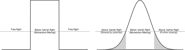
Figure 1. Left: a plane wave with a single energy traversing a square barrier. Even quantum mechanically, it is clear which portions of the trajectory lie in the barrier region and can be called the 'tunneling' portion. Right: the same wave traversing an equivalent Gaussian barrier. Here it is not possible to fully demarcate regions where the trajectory is and is not affected by the barrier.
Download figure:
Standard image High-resolution imageThere is an additional complication when trying to infer the effect of the barrier on the flight time, known as the momentum filtering effect. When considering wavepackets which are a superposition of more than one momentum component, the tunneling process induces a change in the distribution of momenta [4, 45]. Because the probability of tunneling varies with the momentum, and can do so quite drastically (especially for transmitted particles), certain momentum components are more likely to be transmitted than others. For transmitted particles this usually leads to a preference of higher momentum components, for reflected particles of lower momentum components.
This means that for an incident wavepacket, the distribution of momenta that one observes at the screen will be different from the initial distribution. Due to the change in momenta, one would then see a significant change in the flight time of particles transmitted through a static barrier as compared to those transmitted without the barrier. The latter, having a negligible filtering effect, will be lower in energy than the transmitted particles and the time difference between them will grow linearly with the distance of the screen position relative to the barrier potential. Using the free particle flight time introduced here mitigates this masking effect, since the free particle flight time is 'measured' after the scattering is over and thus reflects the momentum filtering.
To summarize, the flight time is an 'asymptotic' tunneling time measure: it involves observing the system far away from the interaction region in both space and time. Qualitatively, we can think of three phenomena that contribute to the flight time: the intrinsic time spent in the barrier region, the time spent in the classically-allowed region discussed above (whether to the left and right of the barrier, or above it, or some combination of the two), and the effects of momentum filtering. As shown below, the momentum filtering contribution can be unravelled and one can answer the question of what the flight time is for crossing the barrier.
The flight time is also a 'direct' measure: it depends only on quantifying the time parameter in the Schrödinger equation itself. Arguably, no time measurement in quantum mechanics is truly direct, as it will always rely on some interpretation and theory. Indeed, much work goes into detector models considering this very problem [46]. However, there is also abundant literature on the detection of single particles in quantum time-of-flight experiments, for instance [38, 39]. The mean flight time described here can be constructed through a simple weighted average of individual time-of-flight measurements—as long as one can measure the time of flight of single particles, the mean time of flight defined here is straightforward to construct. The detector model plays a minimal role and little extra interpretation is needed.
2.3. The flight time in this work
In our computations we use an initial Gaussian wavepacket given by

with an initial mean position x0 < 0, initial width parameter Γ, initial mean momentum p0, and mass M. ℏ is set to 1 such that the wavenumber  is equal to the momentum (M is not set to 1). We restrict ourselves to a symmetric barrier V(q) (square or Gaussian), which is taken to be centered around q = 0 with half-width a. The final measurements are taken at a screen Y > absolute value of x0 after propagation with the propagator
  for time t long enough to ensure almost all of the transmitted wavepacket passes the screen. For the definition of the free particle flight time tFP,T in our previous work, the time of flight for a free, classical particle
  was modified slightly, with p0 being replaced with
  , where
  was the wavenumber solution of a differential equation derived from a steepest-descent approximation. In other words, the mean flight time of the transmitted particle was compared to the time-of-flight of a free particle with the steepest-descent filtered momentum a tunneled particle would have. Equivalent quantities were defined for the reflected distribution by replacing Y with −Y throughout. The steepest descent density decays exponentially so that the mean flight time remains well-defined.
In this present work, we introduce an improved, different way of determining the free particle mean flight time, tFP,T: we calculate ⟨t⟩T(Y), the mean flight time of the transmitted (or reflected) time at the screen Y, and then we also calculate ⟨t⟩T(Y + ΔY), the mean flight time at a slightly further distance, both using equation (4). Since the screen location Y is far away from the barrier, the flight from Y to Y + ΔY is free, and a particle traversing this distance does so with the altered velocity profile it acquires from the interaction with the barrier (with a constant mean velocity). Thus the filtered free particle time is taken as:

and an equivalent definition for tFP,R:

These definitions have the advantage that they can be derived directly from the time-dependent wavepacket. Hence the same type of calculation—taking time means of the transmitted distributions in a numerical simulation of wavepacket propagation—is used to calculate both the tunneling and free particles' times of flight, and there is no need to use an approximate steepest-descent calculation.
We note that the filtered free particle time also includes the portion of the particle moving from the left of the barrier to the barrier. The reason for this is that the filtered time is a post-selection which selects the components of the momentum which are larger. Those components are not limited to being to the right of the barrier.
At this point, we can define a 'TFT' as the difference between the flight time of the transmitted or reflected particle and its associated free particle mean flight time as defined above:

In our previous work we defined a barrier traversal time ttrav in a similar way to equation (9) (including a different definition of tFP,T). It should be stressed though that the name 'TFT' is only valid for square barriers. For smooth barriers such as the Gaussian barrier studied here, the TFT is in reality the barrier crossing flight time, since as already discussed one cannot distinguish between the contributions of the classical allowed and disallowed regions of the potential when considering wavepackets.
2.4. The phase time
The flight time is defined for wavepackets. For stationary states of the Hamiltonian there is no time evolution and thus no flight time. In contrast, the phase time is defined specifically for stationary states, which are of course monochromatic in energy. At a given energy, the transmitted and reflected amplitudes are written as

The phase times are then defined as

for  . The phase time is an indirect measure of the tunneling time—it is obtained by observing a phase shift in the wavepacket due to the interaction with the barrier. It is interpreted as a time difference between the actual time of traversal and that of a free particle time of traversal, which is well-defined for a monochromatic wave. Of course, in both cases, the times are constructs and are not physically directly measurable. This is because the time variation of a stationary state, by definition, is null.
2.5. Phase time vs tunneling flight time
It has been argued by many authors that the momentum filtering effect makes any realistic measurement of the phase time as a flight time impossible [47, 48]. As discussed, the TFT is defined as the difference between the time of flight of a particle that interacts with the barrier and one that does not. This is similar in spirit to the concept of a phase shift, and thus it is not surprising that in our previous work, we found that in the limit of the wavepacket's energy width tending to zero, the TFT coincided with the reflected phase time τΦR(k) [1, 4] (also called the Wigner time [21]), the derivative of the phase shift.
The equality ttrav = τΦR held true for both square and Gaussian barriers as the momentum width tended to zero (with τΦT = τΦR for a Gaussian barrier), and it should hold for any symmetric barrier. In the case of the square barrier, which can be computed exactly [44, 49], the reflected and transmitted phase times differ from each other by the quantity  , which is the time taken for a free particle to traverse the barrier's length. In our previous paper, we showed that τΦR(k) is the time the particle takes to traverse the barrier, refuting several common counter-arguments against the use of the phase time in this manner. In the square barrier case, it is possible to unambiguously demarcate time spent inside the barrier from time outside the barrier, making this identification possible and making it possible to say ttrav = τΦR. For more general symmetric barriers, this demarcation is not possible, and so identifying τΦT as being the time difference due to the barrier and saying tTFT = τΦT is the best that is achievable.
Figure 2 is an updated version of figure 8 from [22], based on equation (9) as defined here. Similar values of the parameters (in atomic units) to the ones used in the previous work are used here: ℏ = 1, M = 158 426, a = 17371.1, V = 3.502 19 × 10−13, p0 = 2.8656 × 10⁻⁴, and in the simulations in the code wavepacket [50] used to generate the wavefunctions, x0 = −429 912, Y = 859 826, Y + ΔY = 950 000. The general behavior is still the same, and the definition converges to the phase time as Γ tends to 0. One notable difference is that the reflected time varies considerably less with Γ. This is due to the definition of the free particle flight time introduced in this paper, which, as already mentioned, includes in it in a time-averaged way the momentum filtering effect. For the same reason, the slope of the transmitted time is significantly smaller than that shown in figure 8 of the previous paper. The phase time τΦT(k) was calculated by numerically differentiating the transmission amplitude generated using a method presented in [51].

Figure 2. The transmitted TFT as defined in equation (9) (closed circular points and overlapping line), the equivalent points for the reflected component (closed square points and overlapping line), and the transmitted phase time for a Gaussian barrier τΦT are plotted as functions of the incident wave-packet width parameter Γ in inverse-square Bohr radii ( ). The lines of best fit are produced using the first five points of each data set, assuming the intercept equals the phase time. The open circular and open triangular points with error bars are the experimentally reported transmitted and reflected times of Spierings and Steinberg [13], respectively, at the experimental Γ and the same mean incident energy.
Download figure:
Standard image High-resolution image2.6. Dwell times
Like the TFT, the phase time is an asymptotic quantity: it is only possible to define a transmission or reflection amplitude asymptotically, and both metrics involve observing the system far away from the interaction region in both space and time. The TFT and phase time have this property in common with other tunneling time definitions such as the Pollak–Miller imaginary time [52]. By contrast, a different set of definitions of the tunneling time are local, since they are based on features of the wavefunction within and around the interaction region. A well-known example is the dwell time [4, 19], τD, which, for a wavefunction in the time-dependent picture, interacting with a square barrier that extends from −a to a in the spatial q coordinate, is defined as:

where the operator  is localized in the barrier region.
Like the flight time, this definition is a direct measure of the tunneling time, as it involves an integral over time of the wavefunction's absolute value squared. As may be inferred from equation (14) below, it can be obtained as a simple weighted sum over individual time-of-flight detection events.
Since the dwell time definition relies on local quantities, it is unable to distinguish between the transmitted and reflected portions of the distribution. One cannot infer the amount of time the transmitted particles spend in the barrier if the transmitted particles cannot be distinguished from the reflected ones. Steinberg proposed a way to bypass this limitation based on weak value theory [27]. His central idea was to define a transmitted and reflected dwell time, whose mean is the dwell time of equation (12). However, as discussed in the
At a fixed energy (with vanishing momentum variance of an incident wavepacket) and (for simplicity) for a symmetric barrier, the dwell time is defined as the ratio of the density in the barrier region to the incident flux ( is the flux operator):

where the Dirac δ function localizes the trace operation to the energy shell. One then finds that the dwell time and the phase times are related by the expression [55]

The last term on the right-hand side is called the 'self-interference' delay τI. This expression amounts to defining the dwell time, a local quantity, in terms of asymptotic quantities only, and it involves combining the transmitted and reflected phase times to make one dwell time.
2.7. Larmor times
The Larmor time experiment was originally formulated for a square barrier potential with a constant (weak) magnetic field localized to the barrier region only, pointing in the z direction. The field induces a Larmor spin precession of angle θy
and frequency ωL. For an incident particle with spin  initially polarized along the x-axis of the Bloch sphere and transmitted along a barrier in the y coordinate, the field induces a change in the spin polarization of the transmitted or reflected particle which is then interpreted to be proportional to two time constants defined by:

and

These two times are local quantities—they measure the change in spin due to the interactions with the barrier, which is an interaction local to the barrier region [24].
Rybachenko [25] describes the y-component of the time as the time a particle takes to traverse the barrier, whilst Büttiker related the z-component to a measure of the strength of the backaction of the measuring device on the particle in the weak-measurement framework [27]. τzT has also been interpreted as a spin rotation due to the barrier height the spin sees differing with orientation [56]. Hauge has argued that τzT should not be thought of as a time at all, but rather as a susceptibility—a sensitivity of the transmission probability |T(k)|2 to changes in energy [33].
In his foundational paper on the Larmor time experiment, Büttiker showed that when the field is sufficiently weak, the two times are related to the phase φT of the scattered particle such that

and

where the derivatives with respect to the barrier height V are evaluated at the actual barrier height (and with equivalent definitions for the reflected amplitude R(k, V) and τyR and τzR). It was later shown that similar definitions hold also for other types of barrier [56–58]. The reflected counterparts have equivalent definitions, and indeed τyT = τyR. Henceforth, we will also refer to τyT as the Larmor phase time.
It is notable that τyT is almost identical in form to equation (11), with a sign change and the derivative with respect to E being replaced with a derivative with respect to V. This is due to the fact that the amount of spin rotation under the barrier depends on  [23]. Similarly, τzT has the same form as the Pollak–Miller imaginary time, except that the derivative of the probability is with respect to the barrier height instead of the incident energy. It is due to this analogy that the Larmor times τyT and τyR are related to the dwell time as in equation (14).
Steinberg noted that when the magnetic field is sufficiently weak, the Larmor times may be considered as weak values of a dwell time. In the Larmor experiment, measuring the transmitted particles implies that the post-selected wave function ψT(q, t) (defined in equation (A2) in the

with a similar definition for the reflected dwell time τD,R. Furthermore, if the incident Gaussian wavepacket may be represented in the momentum space as

then the overlap of the post-selected transmitted wavefunction with the time evolved wavefunction is

where the notation  suggests that this is an averaged transmission amplitude. In the case of the Gaussian incident wavepacket used here, it depends on the incident momentum k0 and width Γ of the wavepacket. A similar property holds for the reflected case.
Operationally, Steinberg claimed that these weak-valued times may be expressed in terms of the time-dependent wavefunction Ψ(x, t) (Brouard et al performed similar calculations without invoking weak value language [32]). For a Gaussian barrier and the experimental setup used in Ramos et al's work, Steinberg et al's operational expression for the transmitted dwell time is

while the reflected dwell time is

Other authors have proposed alternate ways of separating the dwell time into transmitted and reflected components, including by applying multiple projection operators [59], and by using Wigner functions [32]. Indeed there are potentially infinitely many ways of defining weak dwell times [59]. Here we will explore the definitions of equations (22) and (23). However, as noted in the
It must be emphasized that the Larmor times are indirect, asymptotic definitions: measuring something other than time, and depending on the transmission and reflection amplitudes. It is clear that for this definition, an extra layer of derivation is needed to construct a time quantity from the observations as compared to the flight and dwell times discussed above.
They are also monochromatic: they are only well-defined for plane waves or wavepackets with a negligible momentum width. Whilst it can be argued that the times defined in equations (22) and (23) are equally applicable to the tunneling of wide-in-momentum wavepackets, in that case it becomes less clear what their relationship to the definitions of the times in equations (17) and (18) is.
The equivalence between the dwell and Larmor times is still somewhat controversial, with some claiming that this relationship is unique [60] and others asserting that it is not unique [31]. The relationship between the Larmor and dwell times has also been studied and compared to Steinberg et al's work in the contextual values formalism [56].
2.8. Comparing definitions
Just as in our previous work where we showed that the phase time coincided with the flight time at sufficiently narrow values of Γ, in this work, we show that in the same limit, the transmitted dwell time τD,T as defined in equation (22) coincides with the Larmor phase times of equations (17) and (18), which are defined for the square barrier. This is shown in figure 3, which compares numerical calculations of the TFT using equation (9) with the phase time (equation (11)), and compares numerical calculations of the real components of the transmitted and reflected dwell times calculated using equations (22) and (23) with the Larmor phase time of equation (17). (The wavenumber value corresponding to the barrier height  is indicated by the vertical line in all the plots.) The TFT and phase times were found to closely match, as were the weak value dwell time components and the Larmor phase times.
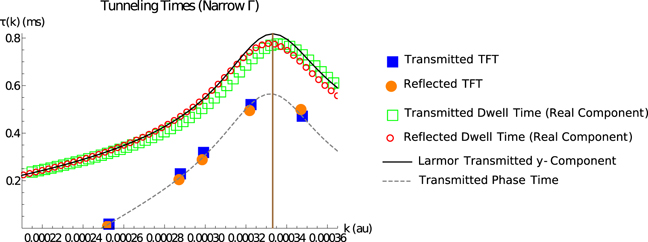
Figure 3. Comparison of the monochromatic transmitted phase time (in milliseconds) with the transmitted and reflected flight times for narrow Γ as a function of the wavenumber k (in atomic units), alongside a comparison of the monochromatic transmitted Larmor phase (y) times with the real components of the transmitted and reflected conditional dwell times for narrow Γ as defined in equations (22) and (23).
Download figure:
Standard image High-resolution imageA similar plot, not presented here, was made comparing the imaginary components of the transmitted and reflected dwell times with the derivative of equation (18), and it was similarly found that the derivatives closely matched their transmitted and reflected weak dwell time counterparts. The wavefunctions as functions of space and time were calculated numerically using the code wavepacket [50], and the transmitted and reflected amplitudes were calculated by numerically solving for them (monochromatically) with a separate scheme from [51].
The parameters used in figure 3 are similar to the ones used in the experiment of Spierings et al and the same as used in figure 2 here, with Γ = 6.796 49 × 10−11. In figure 4, the TFT and weak value dwell time calculations are shown for a larger value of Γ, Γ = 6.796 49 × 10−10 atomic units, which is closer to the value used in the experiment. The reflected and transmitted components of the TFT differ from each other considerably, as do the reflected and transmitted components of the real component of the weak value dwell time.

Figure 4. Transmitted and reflected flight times (in milliseconds) for experimental-width Γ as a function of the wavenumber k (in atomic units), alongside the real components of the transmitted and reflected weak value (Larmor) dwell times for the same Γ.
Download figure:
Standard image High-resolution imageOne reason for this difference is momentum filtering [16, 61], which has a larger impact on wavepackets with wider momentum widths. Due to the fact that the transmission tunneling probability is usually exponentially sensitive to the incident energy while the reflection probability is not, the transmitted component is altered considerably more than the reflected one in the wide-Γ regime for both the dwell time and the TFT. More quantitatively, a steepest-descent calculation [61] can be used to show that the magnitude of the momentum-filtering effect depends on the derivative of the transmission and reflection coefficients with respect to k. Since the transmission coefficient varies more with k over this region, the momentum is more strongly filtered for this component. Another reason for the difference has to do with above-barrier momentum components, since even in the narrow-Γ plot, the difference between the dwell time and Larmor time in the calculations differs the most near the top of the barrier.
The actual experimental data points presented by Spierings et al in [13] do not precisely match the numerical calculations of τy,T etc provided in the same work and re-created here. The authors claim that this is due to undetected asymmetries in the 'barrier' used in the experiment. But it could also be in part due to the momentum filtering and above-barrier effects we discuss here, as well as the actual validity of equations (22) and (23) for computation of the weak value dwell time, as discussed in the
The comparisons given in figure 4 are at an energy near to the peak of the Gaussian barrier, where the phase times (energy derivatives) and Larmor phase times (barrier height derivatives) are quite similar. They are still not quite identical, nor should they be expected to be, as they are fundamentally different quantities derived in different ways. If the two quantities are calculated at lower energies, this difference becomes clearer, as demonstrated in figure 5. For the square barrier portion of the figure, the results are calculated by differentiating exact expressions for the transmission and reflection amplitudes [44]. For the Gaussian barrier portion of the figure, the results are calculated by numerically differentiating numerical expressions for the amplitudes obtained using the method of [51] outlined above.
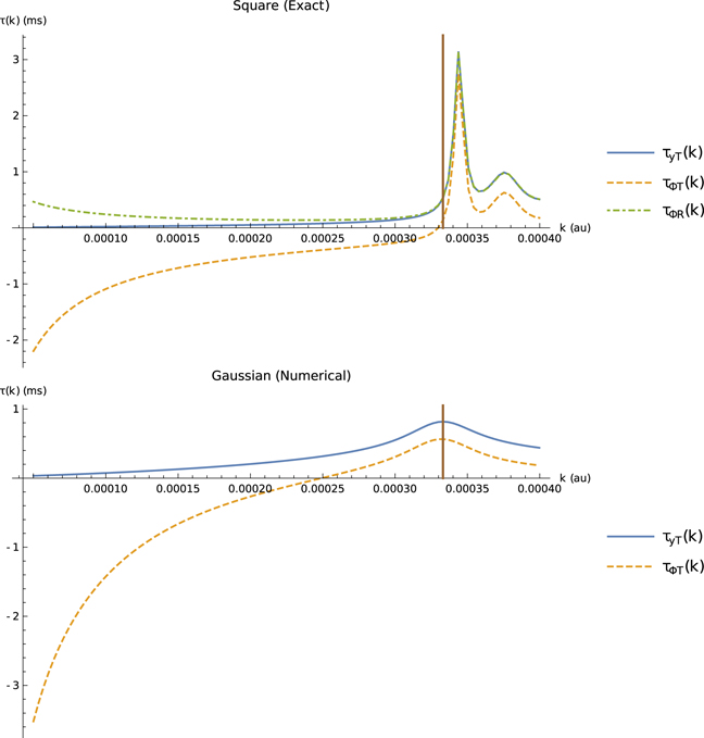
Figure 5. Comparison of the monochromatic transmitted Larmor phase time τyT (in milliseconds) with the transmitted and reflected phase times τΦT and τΦR over a wide range of wavenumbers k (in atomic units) for both square (top) and Gaussian (bottom) barriers. In the Gaussian barrier case, the transmitted and reflected phase times are the same, and so the latter is not plotted.
Download figure:
Standard image High-resolution imageFor the square barrier, the transmitted phase time diverges at low energy, becoming arbitrarily large in the negative direction for sufficiently small energies (which also correspond to the lowest transmission probabilities). The reflected phase time, differing by the quantity  , thus diverges in the positive direction at low energy. The Larmor phase time does not exhibit this behavior, approaching zero as the energy approaches zero. Hauge has noted [33] that tunneling time definitions tend to agree with each other on the order of magnitude of the time measured. Figure 5 is a reminder that this is not always the case.
A summary of the various definitions espoused here is presented in table 1. The quantity ⟨S⟩(y,z),(T,R) is written as a stand-in for e.g.  , where τyT is in principle the same as the quantity defined in equation (17), but is defined in terms of spins as per equation (15), and measured asymptotically. The table is similar to a table by Hauge and Støvneng [1]. We do not comment on the 'extrapolated' phase times cited in that table.
Table 1. The tunneling time definitions discussed in section 2 sorted by whether they depend on asymptotic or local quantities, whether or not they directly measure a time quantity, and whether they are only applicable to narrow-in-momentum wavepackets or can be applied to broader ones, too.
| Time quantities | tTFT,(T,R) | τΦ(T,R) | τD | τD,(T,R) | τ(y,z),(T,R) | ⟨S⟩(y,z),(T,R) |
|---|---|---|---|---|---|---|
| Asymptotic or local? | Asymptotic | Asymptotic | Local | Hybrid | Asymptotic | Asymptotic |
| Direct or indirect? | Direct | Indirect | Direct | Direct | Indirect | Indirect |
| Broad or narrow? | Broad | Narrow | Broad | Narrow | Narrow | Broad |
3. Discussion
3.1. Defining the question
The experimental work by Spierings et al that we examine here represents a significant step forward in the measurement of the dynamics associated with quantum tunneling. The remarkable ability to experimentally observe metrics formalized almost 40 years ago by Büttiker and others forces us to re-open questions about their interpretation.
An underlying motivation of many of these studies is the question 'how long does it take a quantum object to tunnel through a barrier?' But this question is ill-posed. It is not possible in general to demarcate the tunneling and non-tunneling regions of a wavepacket's motion in a quantum regime [31, 32, 62]. Outside of Bohmian mechanics or Feynman path integral formulations of quantum mechanics [63–65], the only instance where this demarcation is possible is in the example of a square barrier (or similar variants). For more general barriers like Gaussian-shaped ones, the distinction cannot be made unambiguously, even when considering Wigner-phase-space formulations [20, 59], and even for monochromatic plane waves. The notion of a particle being 'inside' a barrier is an inherently classical concept. The question which should instead be addressed is: how long does it take a quantum particle to cross a barrier?
Due to these issues, we argue that the TFT defined in equation (9) is the 'natural' way to answer this question. The flight time is, in principle, experimentally measurable. It is determined directly by the time-dependent Schrödinger equation. It is possible to obtain all necessary information from the asymptotic behavior of the wavepackets. It is applicable to wavepackets with large momentum-space widths and with significant above-barrier transmission, and to near-arbitrarily-shaped barriers. Provided that the mean of the incident wavepacket's position can be defined sensibly, it gives a clear, physically-sound estimate of the time associated with the interaction with the barrier. This is demonstrated here, and in our previous paper [22], where we also argue against concerns about the transmitted wavepacket not being causally connected to the incoming one.
3.2. Properties of 'tunneling times'
The issue is not merely a conceptual one: not only do the different definitions of the time differ from each other in magnitude, they can have different physical properties, too. Since we show that the phase time can be thought of as the difference in time of flight between a tunneled and free particle, the fact that the phase time becomes arbitrarily large in the negative direction suggests that it is possible for tunneled particles to arrive ahead of free ones. We discussed the implications of this for relativity in a previous work [37].
The Larmor phase time is different. It tends to zero at low energy, rather than diverging to negative infinity. Its physical interpretation is also different. It is defined in terms of Larmor precession. Experimentally, the time is obtained by counting how many particles have spins in certain directions before and after a collision via equations (15) and (16). At no point is an actual time measured experimentally—at best, it is an indirect tunneling time measure.
This is, of course, a key feature and a huge advantage of the experiment: directly measuring times in quantum mechanical experiments is difficult, and proxy quantities are a useful way of avoiding having to do so. This was one of the motivations for Baz', Rybachenko, Büttiker and others in devising the Larmor experiment in the first place. But since something different is being measured, it does raise the question of the extent to which the change in spin polarization can be interpreted as an actual time spent inside a barrier, as claimed in many of the works discussed here. To further emphasize this point: there are, in fact, many ways to elucidate a 'time' from the Larmor experiment. Büttiker suggested that the tunneling time is  [1, 23], a quantity which, for example, negates the Hartman effect [66]. This is different from the weak value interpretation of Steinberg. There are many other ways to elucidate a time from the spin polarization experiment. Which is 'correct'?
In a recent paper, Spierings et al claim that [14] 'tunneling takes less time when it is less probable', but this is a natural consequence of defining the tunneling time as being equivalent to the Larmor phase time, since it tends to zero at low energy where tunneling is the least probable (and also decreases as the barrier height is increased). If, as we concluded in [22], one considers the tunneling time to be equal to the reflected phase time, then, in the square barrier case, this is no longer true: figure 5 shows that τΦR increases as k decreases at low energies. The difference between the tunneled and free particle flight times decreases as energy decreases for all barriers, but the tunneling time itself, as we argue it should be defined, does not. One can also show that both the reflected and transmitted phase times decrease as the barrier height increases.
These points can be further emphasized by examining the Hartman effect [4, 66] (sometimes called the MacColl–Hartman effect [67]) for the metrics in question. For a square barrier, the reflected phase time τΦR hardly changes as a function of a, the barrier width, when it is past a certain value of a that varies with k. This 'saturation' of the tunneling time as a function of a is the source of the Hartman effect. This can be seen in figure 6 for the four different below-barrier energies for which the reflected phase time was calculated in figure 3, and for one lower-energy value of k (klow). The results for figure 6 were generated using the same method for square barriers as outlined for figure 5.
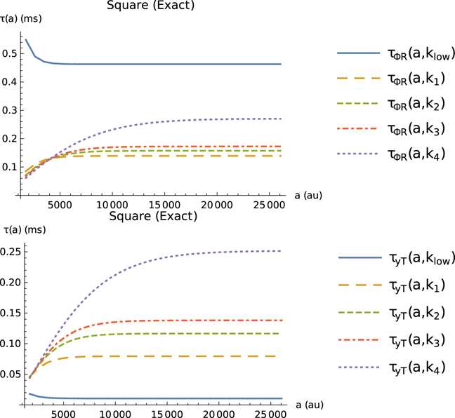
Figure 6. The (monochromatic) reflected phase time τΦR (top) and transmitted Larmor phase time τyT (bottom) for square barriers of varying a, as functions of a, for five different energies. The parameters are as in figure 5. The higher energies are the same as the ones in figure 3, and the lower energy klow = 0.2k1.
Download figure:
Standard image High-resolution imageAlso in figure 6 we show the same plot for the Larmor phase time τyT for square barriers, which has the same 'saturation' property for the energies seen here, since the Hartman effect exists also for the Larmor phase time. Here it is not the tunneling time that is becoming saturated inside the barrier, but the change in spin—a quantity that can be related to a time but is not a time in and of itself. Increasing the barrier width a is also equivalent to increasing the integration range in the dwell time calculation of equation (12) or equation (22), and so the Hartman effect is also considered to be a saturation of the wavefunction density inside the barrier.
In figure 7, we show the phase time and the Larmor phase time calculated for Gaussian barriers as functions of the width. Here, the Hartman effect cannot be directly observed, since the effect of the particle moving in the classically-allowed region of the potential before going 'under' the barrier cannot be disambiguated from the effects of the barrier itself. The figure also shows the extent to which the phase time differs from the Larmor phase time. The Larmor phase time τyT varies with a in a similar way to τΦR in both the square and Gaussian cases for energies close to the barrier top, suggesting that the two time metrics have properties in common. However they clearly behave quite differently at the lowest energy klow, further underscoring the difference between the two tunneling time metrics. The results for figure 7 were generated using the same method for Gaussian barriers as outlined for figure 5.

Figure 7. The same phase times (top) and Larmor phase times (bottom) for Gaussian barriers of varying width a. Other details are as in figure 6.
Download figure:
Standard image High-resolution image
There is one further property of the Larmor experiments which we note. In the limit of a monochromatic (in momentum) wave, the Larmor phase time is well-defined in terms of the scattered phase, whether reflected or transmitted. For incident wavepackets the situation is quite different. The time-dependent wavepacket only approximately predicts the change in the spin polarization. The computation of the weak value associated with the spin polarization, as suggested by Steinberg and as discussed in the
In contrast to the Larmor phase time, the dwell time is a direct measure of the time a particle spends in the barrier region. In the monochromatic limit the dwell time is related to the reflected and transmitted phase times as in equation (14). For a general wavepacket, as may also be seen from equation (12), it is obtained directly from the time-dependent wavefunction. From a formal point of view, it is well-defined as a strong value of a dwell time operator. The difference between the dwell time and the phase time or the flight time is that the latter two answer the question of what the interaction time is of transmitted (or reflected) times with the barrier. The dwell time does not distinguish between the transmission and reflection, but only relates to the time spent by a particle in the region of the potential. As such, even though the dwell time does display the Hartman effect, it does not by itself lead to the question concerning superluminal times, since it does not relate the finite time to the transmitted particle.
4. Conclusions
In this work we have studied several common definitions of the tunneling time, and we have:
- Highlighted the importance of the distinction between direct and indirect measures of tunneling times, and classified many definitions in this way.
- Established which definitions are usable only for monochromatic wavefunctions and/or square barriers, versus the ones that may be used for wavepackets and/or more general barrier shapes.
- Introduced a novel definition of the free particle flight time which does not suffer from ambiguities related to long-time tails and is obtained directly from the time dependent wavefunction.
- Argued for the TFT as the most general and meaningful way to assign a time-related quantity to a tunneling event, and continued discussions we have presented about the implications of this for phenomena such as the Hartman effect.
- Developed our previous work exploring the connections between the flight time and the phase time, with improved and updated definitions.
- Expanded that work to also explore the similar connections between Larmor times and weak dwell times, demonstrating that the two can only be connected in the narrow-wavepacket limit.
- Placed these studies in the context of recent experimental results that used Larmor times, to identify the places where there are dissonances between the experiment and the theory that supports it.
To conclude, it must be said that even for intrinsically quantum processes, like tunneling, or spin-flips, it is tempting to invoke classical language when describing them. It is also tempting to extend that classical language and impose classical concepts on those processes. This explains much of the controversy surrounding tunneling times. Even in one dimension, there are countless complications surrounding a quantum particle scattering off a barrier. As such, it was inevitable that a plethora of different tunneling time measures emerged over time.
The recent advances in experimental techniques have come close to elucidating the Larmor phase time but even this has not yet been achieved experimentally, due to the finite width of the incident wavefunction. The final and perhaps central conclusion of this paper is that a measurement of the flight time is needed to push forward the frontiers of this field of research.
Acknowledgments
This work was supported by Grant 408/19 of the Israel Science Foundation.
Data availability statement
All data that support the findings of this study are included within the article (and any supplementary files).
Appendix.: The Larmor experiment and weak dwell times
Conceptually, the Larmor experiment is one in which the magnetic field in the interaction region is weak so that it hardly disturbs the particle as it traverses the barrier region. Furthermore, the results of the experiment are a separate measurement of the change in spin polarization of reflected and transmitted particles. The experiment post-selects the state being measured. As noted by Steinberg, these are precisely the two properties that define a weak measurement whose result is expressed in terms of a weak value [27].
Specifically, following Steinberg [27], we denoted in equation (19) the post-selected transmitted (reflected) state |ψT⟩ (|ψR⟩) and the associated weak dwell time values. What precisely are these post-selected states? For the Gaussian incident wavepacket of equation (6), the bandwidth function Φ(k), introduced in equation (20), is

Steinberg defines the post-selected transmitted wavefunction ψT(q, t) as

where ψk (q) is the eigenfunction of the scattering Hamiltonian of equation (1). The post-selected reflected wavefunction is defined analogously

Asymptotically, the eigenfunctions outside of the potential interaction region are

It is then a matter of straightforward algebra to show that for sufficiently long times such that the scattering event is over, the overlap of the transmitted (reflected) post-selected function ψT(q, t) (ψR(q, t)) with the time-evolved wavefunction Ψ(q, t) has the property


Steinberg then proceeds to consider the weak value of the transmitted and reflected dwell times defined as in equation (19), and claims that their mean is the dwell time as in equation (12). Specifically, the claim is that

This result, however, is only true if  and
and  also hold, but this is not the case. This may be seen by applying the equation to the definitions given in equations (22) and (23). Only in the limit that Γ → 0 is the unitarity condition correct. Note that this comment is not novel: it is a natural consequence of considering conditional dwell times, as studied in some detail in [32]. There is a real difference between computing theoretically the spin polarization caused by a wavepacket and being able to interpret it as a conditional dwell time in the sense of obeying equation (A7).
Steinberg also relates the post-selected functions to the time-dependent wavefunction Ψ(q, t) via equations (22) and (23). This, too, is correct when the bandwidth function is sufficiently narrow such that  and
and  , but not otherwise. Computation of the post-selected states as defined in equations (A5) and (A6) necessitates knowing the eigenfunctions of the Hamiltonian in all space. This is much more involved than computation of a single time-evolved wavefunction Ψ(q, t). In this context we do note that some work has been done on the wavepacket version of this problem [68–70].
Finally, it is worth noting that Steinberg's definition of the conditional dwell times is a hybrid scheme that contains local and asymptotic elements—the integrals over the barrier region, and the transmission and reflection amplitudes respectively. It is also a hybrid of direct and indirect measurements. The conditional dwell times are weak values and so in general are complex-valued.