


Abstract
We formulate the effective Hamiltonian of Rashba spin–orbit coupling (RSOC) in  (LAO/STO) heterostructures. We derive analytical expressions of properties, e.g. Rashba parameter, effective mass, band edge energy and orbital occupancy, as functions of material and tunable heterostructure parameters. While linear RSOC is dominant around the Γ-point, cubic RSOC becomes significant at the higher-energy anti-crossing region. We find that linear RSOC stems from the structural inversion asymmetry (SIA), while the cubic term is induced by both SIA and bulk asymmetry. Furthermore, the SOC strength shows a striking dependence on the tunable heterostructure parameters such as STO thickness and the interfacial electric field which is ascribed to the quantum confinement effect near the LAO/STO interface. The calculated values of the linear and cubic RSOC are in agreement with previous experimental results.
Export citation and abstract BibTeX RIS

Original content from this work may be used under the terms of the Creative Commons Attribution 3.0 licence. Any further distribution of this work must maintain attribution to the author(s) and the title of the work, journal citation and DOI.
1. Introduction
In the search for a novel platform for spintronics devices, oxides heterostructures has emerged as one of the most promising candidates due to their excellent electrical and magnetic properties [1]. The formation of two-dimensional electron gas [2–5] and magnetism [6–10] at the interface of transition metal oxides such as  (LAO/STO) gives rise to a unique opportunity to study and implement spintronics in a single platform [11].
A key requirement to spintronics application is the presence of spin–orbit coupling (SOC). As the inversion symmetry at the interface of the two transition metal oxides is inherently broken, there exists SOC of Rashba type [12–14]. Magnetotransport measurements have detected a substantial spin–orbit splitting of 2–10 meV at the LAO/STO interface [14–17], while a much stronger spin-splitting of 90 meV has been observed on the surface of STO [18]. Strikingly, the spin splitting is not just of k-linear [14] but also k-cubed Rashba types [19]. Furthermore, the interfacial Rashba coupling is versatile, and can be tunable via electrical gate [12–14], and via crystal orientation selection [20–22]. For comparison, the above splitting is higher than that of 1–5 meV in typical semiconductor heterostructures [23]. The strong Rashba coupling in LAO/STO has led to the realization of various spintronics effects such as spin-to-charge conversions [24–28] and spin–orbit torques [29]. The fact that these phenomena are interfacial in nature allows us a much better degree of external control of its electrical and magnetic properties compared to conventional spintronic materials such as ferromagnetic metals [30, 31]. More importantly from the application standpoint, the conducting layer is protected against external perturbations as it is sandwiched between conventional oxides insulators [30, 31], which makes it more robust in comparison to the exposed surface states of topological insulators.
At the same time, theoretical models have been proposed to elucidate the rich SOC properties of the STO-based heterostructures, which are not captured by the standard linear Rashba theory [32]. Combined first-principles calculations and tight-binding approach [13, 33, 34] revealed a multi-orbital Rashba effects, of the linear and cubic types, at the LAO/STO interface layer. Nevertheless, the crystal field, one of the ingredients of the SOC which accounts for the properties of the heterostructure, had been deliberately introduced, and the contribution of the bulk STO as well as the inter-orbital hopping was ignored. Significantly, the large spin splitting at the anti-crossing region, a signature of the multi-orbital effects, has not been fully elucidated. Recently, a theory based on k.p model [35, 36], including the contribution of the bulk STO, predicted a spin splitting induced by the inter-orbital hopping and interfacial band-bending. However, a complete picture of the multi-orbital Rashba SOC is still lacking.
In this work, we aim to construct the effective Hamiltonian of Rashba spin–orbit coupling system in STO-based structures, taking into account the underlying factors such as the confinement effect, as well as interface effects including inversion symmetry breaking (ISB) and band-bending. We derive analytical expressions of properties, e.g. Rashba parameter, effective mass, band edge energy and orbital occupancy, as functions of material and tunable heterostructure parameters. We show that the type and strength of spin–orbit coupling as well as the orbital selectivity are tunable by controlling geometric factor such as STO thickness and by applying electric field via gate voltage. The thickness and gate control of SOC provides a possible avenue for optimization of Rashba SOC for spintronics applications and devices.
2. Model
We consider a 2DEG system in STO-based heterostructure. The 2DEG can be generated by interfacing STO with either LAO [37] or vacuum with δ-doping [22]. In the low energy limit, the electron in bulk STO is described by following Hamiltonian

In the above  is the kinetic energy of the d-electron in the
  band in cubic crystal,
  is the inter-orbital hopping,
  is the atomic spin–orbit interaction, and the last term is the electrical confinement potential in the z-direction
  .
.
In the t2g orbital-spin basis  , with yz, zx and xy representing the dyz, dzx, and dxy orbitals, respectively, the electron in the bulk Ti t2g band can be described by the effective
  Hamiltonian [35, 38]

where  is 2 × 2 unit matrix. The diagonal terms of
  is given by
  and the off-diagonal terms are
  , with effective mass parameters L, M, N, and
  . The other elements follow by exchanging the x, y, and z indices. In the above, the off-diagonal elements can be considered as the inter-orbital hopping in the bulk STO. The fit of the
  model to the energy dispersion from our DFT calculations yield the mass parameters as
  , and
, and  (see appendix A for the details).
At the same time, in the presence of interface, the inversion symmetry is broken which leads to an additional Hamiltonian [34, 39–42]
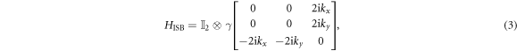
up to the first order in k, where γ is the ISB parameter. In general, the ISB parameter is position-dependent, having a maximum value at the interface and rapidly decreases across at the deeper layers [41, 42].
The above Hamiltonian is symmetrical with respect to the xy, yz, and zx orbitals. However, this orbital degeneracy will be lifted in the presence of the atomic SOC. The SOC splits the six-fold degeneracy into a four-fold J = 3/2 multiplet of symmetry  and a twofold J = 1/2 multiplet of symmetry
  . In the original t2g basis, the SOC is expressed as

where the SO splitting is calculated via DFT to be  (see appendix A).
3. Effective Hamiltonian
We now turn to derive the Rashba split band structure of a STO-based heterostructure with 2DEG. For a STO film with finite thickness, we first find the eigen-states of (B2) at the Γ point  . Subsequently, an effective Hamiltonian at other k values can be obtained by projecting the full Hamiltonian into the space of these eigenstates.
To simplify the analytical calculation, we transform the Hamiltonian into the basis  of
of  and
and  multiplets ,
  , in which the atomic SOC matrix in equation (4) is diagonalized (see appendix B). In the above basis, the Γ-point Hamiltonian is block-diagonalized and it can be decomposed into three subsets as
  , where

in which  ,
,  , and
, and  .
.
For STO slab with finite thickness d, the electron states are quantized along the  direction, and we can make a substitution
  . The eigenvectors and subband energies of electron can be found by solving the Schrödinger equation
  in which ψ(z) is six-component eigenvector.
In solving the above Schrödinger equations in a STO slab with finite thickness d, we assume that the electron is confined in a quantum well with open boundaries, i.e. ψ(z = 0, d) = 0. This assumption may be understood by considering the character of the boundaries. On the one hand, at the LAO/STO interface, the La t2g states in LAO layer lie far above the Ti t2g states in the STO layer [5]. Therefore, the penetration of the Ti t2g states into the LAO can be neglected [5] and one can assume an infinite barrier at the interface for the simplicity. On the other hand, the other surface of the STO slab is open to vacuum, and thus an infinite barrier potential is imposed. Similar boundary conditions are also applied for the δ-doped STO slab, where both STO surfaces are open to vacuum.
In the framework of variational approach, the solutions are given by  and
and  where the spatial envelope functions read as

Here,  , Cτ is the normalization constant, and βτ is the variational parameter for the minimization of the corresponding eigen-energy
  , where
  is the eigenvalue energy solution when V = 0 given by
 ![${E}_{0}^{(0)}=M{\lambda }^{2}-{\xi }_{\mathrm{SO}},{E}_{\pm }^{(0)}=\tfrac{1}{2}\left[{\xi }_{\mathrm{SO}}+(M+L){\lambda }^{2}\right]\pm \tfrac{1}{2}{{\rm{\Delta }}}_{I}$](https://content.cld.iop.org/journals/1367-2630/21/10/103016/revision2/njpab4735ieqn38.gif) , in which
, in which

with  , and F(β) is the correction when
  (see appendix B for details).
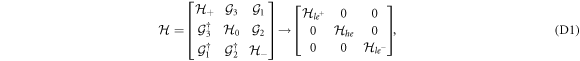
Rearranging the sequence of the six eigenvectors as  , and by projecting the full Hamiltonian to the spin-orbital space of these vectors, we obtain an effective Hamiltonian beyond the Γ-point in block form as (see appendix C for the full expression)

In the above, the diagonal blocks are given by (for τ = 0, ±)

which are characterised by bottom band edges Eτ, effective masses  , and Rashba parameters ατ. Here,
  is the electron momentum in the x–y plane,
  is the vector of the Pauli matrices, and
  is the unit vector perpendicular to the STO slab.
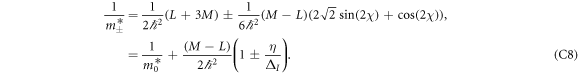
First, we look at the effective masses given by  Recall that M > L, and η/ΔI < 1, we have
  , which indicates that
  describe light-electron (denoted as
  ) bands, whereas
  corresponds to the heavy-electron (he) band. Furthermore, it can be verified that E+ > E0 > E−, so that the two le-bands are sandwiched by the he-band. This arrangement leads to the anti-crossing between the bottom (le−)and the middle (he) bands (see figure 1(a)).

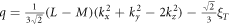
Figure 1. (a) Band structure obtained from the full effective Hamiltonian includes two light electron bands (le±) sandwiched by a heavy electron band (he). (b) The corresponding spin-splitting as function of momentum. (c)–(d) Energy contours and spin textures at different Fermi level: near bottom edge of the le− band (orange dashed line), the spin splitting is of linear Rashba type with characteristic spin orientations along the isotropic energy contours (d); whereas close to the crossing region (green dashed line), substantial cubic and higher order spin splitting yields anisotropic contours and deformed spin textures(c). (e) Orbital polarization defined in equation (17) represents the orbital character in each band: dxy and dyz/zx are predominant around Γ-point in the le− and he bands, respectively, whereas they are more equalized close to the crossing point.
Download figure:
Standard image High-resolution image3.1. Linear Rashba SOC
Now let us consider the expressions of linear RSOC given by

where ΔI is given in equation (7) regarded as effective crystal field, and

is considered as the effective inversion-symmetry breaking, with the integration taken over the STO slab. In the above,  is the spatial distribution function, thus
  is the average ISB parameter across the STO slab. As the ISB constitutes an interface effect, it is only finite near the interface layer, and becomes vanishingly small in the bulk [41, 42]. Thus, equation (11) indicates that the localization of electron at the interface is significant for inducing large effective ISB, which can be achieved by having a large confinement effect induced by external electric field and/or charge density [43]. To obtain a simple analytical expression of the average ISB parameter, we consider the case where the ISB is finite only at the interface layer and zero elsewhere in the bulk, i.e.
  , where θ(x) is the Heaviside step function, and a = 3.870 Å is the lattice constant of STO crystal. In this case, the average ISB parameter evaluates as

in which 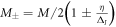 . Equation (12) shows that the average ISB, and thus the RSOC, is scaled with the interface confining electric field
  to the first order as depicted in figure 2(c).
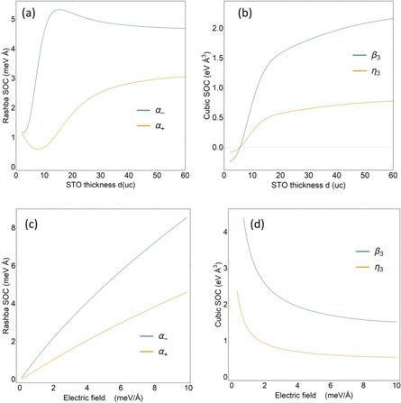
Figure 2. Dependence of the linear and cubic SOC parameters on STO thickness d when  (a)–(b), and on electric field
  when d = 50 Å (c)–(d).
  are the linear RSOC parameters of the light electron bands (le±), respectively, and β3, η3 are the cubic SOC parameters of the heavy electron band (he).
Download figure:
Standard image High-resolution imageFurthermore, it can be seen that reducing the QW width d (STO thickness) will increase the effective ISB due to the wavefunction localization near the interface. However, the effective crystal field in the thin film limit reads as

which also increases with decreasing d. This trend is ascribed to the quantum confinement effect in the STO quantum well, which causes the subbands further split in the thin STO limit. From equation (10), these competing trends above between the effective ISB and effective crystal field lead to non-monotonic thickness dependence of the RSOC (see figure 2(a)). In general, the RSOC diminishes with reducing STO thickness, which is one of our main results.
On the other hand, at large STO thickness, the effective crystal field reduces to  , and
, and  , which result in a saturation of the linear Rashba to
  as shown in figure 2(a). It is interesting to see that in the large thickness limit, the saturation value of RSOC has a weak dependence on the atomic SOC ξSO. However, this does not deny the vital role of the atomic SOC, as the RSOC expression in equation (10) would vanish if ξSO is set to zero in the first place. Assuming typical parameter values, the linear Rashba coefficient is found to be in the range of 1–10 meV Å, corresponding to spin-splitting of 1–10 meV, which is consistent with previous computational [13, 33, 34] and experimental works [14–17].
We note that in other transition metal oxides such as  [44], the atomic SOC is much stronger than that in the
  . However, the crystal field in such oxides is also much larger at the same time [44]. Therefore, following equation (10), the strong atomic SOC oxides does not always translate into a strong Rashba SOC. Experimentally, it has been shown that the Rashba SOC in
  is about 5 meV Å [45], a strength which is comparable to that in the
  .
.
3.2. Cubic Rashba SOC
Now we turn to discuss role of the off-diagonal elements  in equation (8), which describe the coupling between the mj = ±3/2 and mj = ±1/2 states. It has been shown that the above coupling is the prerequisite for the presence of cubic SOC in the mj = 3/2 states [23], which in our case is the he bands. Indeed, by reducing the 6 × 6 Hamiltonian (8) to three 2 × 2 matrices by means of quasi-degenerate partitioning [23], we obtain cubic corrections as


in which the k-cubed SOC parameters are given by

in which  , where we defined
 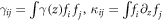 , and
, and  (see appendix D). In equation (16), there are two cubic RSOC terms with different anisotropy in k-space. The first term depends on the mass difference, i.e. M – L, which is responsible for the mass anisotropy in the bulk STO. The second term stems from the the bulk inter-orbital hopping N, which is responsible for the asymmetry in the bulk. The cubic SOC parameters have a similar thickness dependence as in the linear case, in that they saturate at large thickness limit as shown in figure 2 (b). However, the cubic SOC diminishes with increasing electric field, in contrast to the opposite trend shown by the linear RSOC plotted in figures 2(c) and (d). With typical parameter values,, the cubic RSOC is estimated to be in the range 1−4 eV Å3, which is in agreement with previous experimental and computational works [13, 19]. Furthermore, the strength of cubic SOC has been shown to decrease at high electron density [19], a trend which is consistent with our theory taking into consideration the linear correlation between the interface electric field and electron density [43].
3.3. Orbital polarization
In the above, we obtain three pairs of bands, each of which is a mix of dxy, dyz, and dzx orbitals. To analyze the contribution of these orbitals in each band, we introduce the orbital occupancy which is obtained by projecting the eigenstates of the effective Hamiltonian (8) onto the t2g basis states (see appendix E for details). Denote  as the occupancy of orbital i = xy, yz, zx in band
  , we can define the orbital polarization as

which characterizes the contribution of the preferable dxy in the interfacial 2DEG channel. In figure 1(e), the orbital polarization is depicted, which shows drastically different contribution of the orbitals in each band at different energy region. Around the Γ-point, the orbitals are well polarized with dxy and dyz/zx predominant in the two lowest bands, respectively. In this case, the orbital polarization can be obtained as 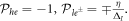 Close to the crossing region, stronger mixing between the dxy-like and dyz/zx-like bands will neutralize the orbital polarization. This trend is consistent with previous computational works [46, 47], where it has been shown that the dxy orbital filling is less at higher energy region. At the same time, the relative contribution of the different orbitals can be controlled by tuning the heterostructure's parameters such as STO thickness. For example, the dxy orbital contribution becomes more dominant in the lowest le− band when the STO thickness is reduced, and approaches
  in the thin limit, whereas its weight reduces as

in the thick limit.
The thickness dependence of the dxy occupancy is in line with the diminishing of the RSOC in the thin limit. The RSOC originates from the ISB, which represents the hopping between the dxy and  at the interface as shown in equation (3). This means that only bands that occupied by both dxy and dyz/zx orbitals will show the linear RSOC. Therefore, in thin STO slabs, the dyz/zx disappears in the le− bands resulting in the vanishing of the hopping as well as the RSOC. Similarly, since there is no dxy in the he bands, the linear RSOC is absent in these bands at all STO thickness. Instead, the he band shows cubic SOC as discussed in the previous section.
4. Conclusion
In this work, we formulate the analytical Hamiltonian of Rashba splitting in the t2g bands of STO heterostructure based on  formalism. First, we express the Rashba parameter as functions of the heterostructure parameters and show that it is thickness dependent. Strikingly, the RSOC diminishes as the STO thickness reduces, and it saturates in thick STO layer. The hybridization between the orbitals results in orbital-dependent Rashba spin splittings. Explicitly, the linear Rashba SOC is associated with the dxy orbital which preferably occupies the lowest band at low energy region. On the other hand, at higher energy crossing region, the cubic Rashba SOC accompanies the enriched dyz/zx orbitals. These results reveal the capability to control the spin–orbit coupling and orbital selection in
  heterostructures for spintronics applications and devices.
Acknowledgments
MBAJ would like to acknowledge MOE Tier I (NUS Grant No. R-263-000-D66-114), MOE Tier II MOE2018-T2-2-117 (NUS Grant No. R-398-000-092-112) grants and NRF-CRP12-2013-01 (NUS Grant No. R-263-000-B30-281) for financial support. This work is also supported by the Ministry of Educations (MOE2015-T2-2-065, MOE2015-T2-1-099, MOE2015-T2-2-147, and MOE2017-T2-1-135), Singapore National Research Foundation under its Competitive Research Funding (NRF-CRP 8-2011-06 and NRF-CRP15-2015-01) and under its Medium Sized Centre Programme (Centre for Advanced 2D Materials and Graphene Research Centre), and FRC (R-144-000-379-114 and R-144-000-368-112).
Appendix A.: Determine  parameters via DFT calculation

To determine the  parameters, first-principles calculations were performed using density-functional theory (DFT) based Vienna ab initio simulation package (VASP5.4.4.18) with local density approximation (LDA) for the exchange-correlation interaction. Projector augmented wave potentials were selected to account for the interactions between electrons and ions. The LDA+U method was used with on-site effective U = 1.2 eV for the Ti d orbitals. The kinetic cut off energy for the expansion of plane-wavefunction was set to 500 eV. Monkhorst–Pack-based k-point grids for sampling the first Brillouin-zone were set to 8 × 8 × 8 and 8 × 8 × 1 for bulk STO and LAO/STO respectively. The Hellman–Feynman forces on each atom were minimized with a tolerance value of 0.01 eV Å–1 for bulk STO, bulk LAO, and
  heterostructure. Based on these settings, the equilibrium lattice constant of the bulk STO is calculated a = 3.870 Å, which is consistent with the experimental result (3.905 Å).
Without atomic SOC—Along k[100], the dispersions are given by ![${{Lk}}_{[100]}^{2},{{Mk}}_{[100]}^{2}$](https://content.cld.iop.org/journals/1367-2630/21/10/103016/revision2/njpab4735ieqn80.gif) . By fitting the calculated energies along k[100] direction to these
. By fitting the calculated energies along k[100] direction to these  formula (as shown in figure A1(a)), we can obtain the values of
  , respectively. Similarly, along k[111] the dispersions are read as
 ![$1/3(L+2M-N){k}_{[111]}^{2},1/3(L+2M+2N){k}_{[111]}^{2}$](https://content.cld.iop.org/journals/1367-2630/21/10/103016/revision2/njpab4735ieqn83.gif) . The different between these two bands are
. The different between these two bands are ![${{Nk}}_{[111]}^{2}$](https://content.cld.iop.org/journals/1367-2630/21/10/103016/revision2/njpab4735ieqn84.gif) , and thus by fitting the dataset to this expression, we obtain
, and thus by fitting the dataset to this expression, we obtain  .
.
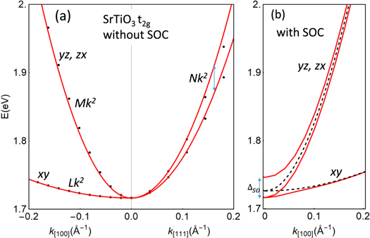
Figure A1. (a) Dispersion of the t2g bands in bulk SrTiO3 obtained via DFT calculation without SOC. The fit of the k.p model to the energy dispersion along [100] and [111] directions yields the mass parameters as  , and
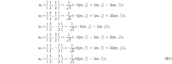
, and  , respectively. (b) Dispersion with SOC shows a splitting of
  meV.
meV.
Download figure:
Standard image High-resolution imageWith SOC—Similarly, in the presence of the atomic SOC, the three t2g bands are no longer degenerate at the Γ-point, and the gap is determined by the SOC splitting ΔSO = 29.85 meV (as shown in figure A1(b)).
Appendix B.: Eigenstates and eigenenergies of the Γ− point Hamiltonian
We introduce  basis given by
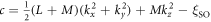
in which the atomic SOC Hamiltonian is diagonalized ![${H}_{{\rm{SO}}}={\xi }_{{\rm{SO}}}\mathrm{diag}\,\left[2,-1,-1,2,-1,-1\right]$](https://content.cld.iop.org/journals/1367-2630/21/10/103016/revision2/njpab4735ieqn90.gif) . The full Hamiltonian in this basis is given by
. The full Hamiltonian in this basis is given by

where
in which  , and
, and  ,
,  ,
,  ,
,  , and
, and 
Schrödinger equations—The Γ−point Hamiltonian is given by

Following the decomposition of the above Hamiltonian, the six eigenstates can be written in general forms as


corresponding to eigen-energies E± , E0, respectively, in which σ = ± stand for  , respectively. In the above, the spatial functions
  and
and  are determined by solving the following coupled differential equations
and f0(z) is the solution of following differential equation

Boundary conditions—In solving the above Schrödinger equations in a STO slab with finite thickness d, we assume that the electron is confined in a quantum well with open boundaries, i.e.  . This assumption may be understood by considering the character of the boundaries. On the one hand, at the LAO/STO interface, the La t2g states in LAO layer lie far above the Ti t2g states in the STO layer [5]. Therefore, the penetration of the Ti t2g states into the LAO can be neglected [5] and one can assume an infinite barrier at the interface for the simplicity. On the other hand, the other surface of the STO slab is open to vacuum, and thus an infinite barrier potential is imposed. Similar boundary conditions are also applied for the δ-doped STO slab, where both STO surfaces are open to vacuum.
Solutions in zero field—First, we find the the solutions of (B7) and (B8) in the absence of the electric field, which can be found as


corresponding to eigen-energies


respectively. In the above, the spatial coefficients are simple sinusoidal functions as

and the spinor angles in equation (B9) are read as

It is easy to verify that  , which secures the orthogonality of the eigen-wavefunctions
  . Furthermore, this angle is in the range
  .
.
Solutions under applied field—In the presence of the confinement potential  , with
  being the electric field, the solutions can be found via variational method [48], in which the eigen wavefunctions are expressed as


in which

where Cτ are the normalization constants given by

and βτ are the variational parameters for minimization of the corresponding energies

in which

where M0 = M, and  .
.
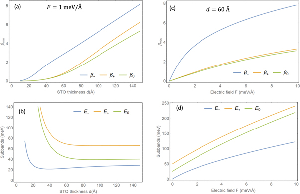
The variational parameters can be obtained by minimizing the above energies, which increase as the electric field and the well width increase, as depicted in figure B1. In the limit of weak electrostatic energy  , the variational parameter and corresponding energy can be approximated as

On the other hand, in the strong electrostatic energy limit δ ≫ 1, we have

Figure B1. The variational parameters and subbands energies as functions STO thickness when  (a)–(b), and as functions of electric field when d = 60 Å (c)–(d), respectively.
Download figure:
Standard image High-resolution image
Appendix C.: General effective Hamiltonian
Having derived the general expression of the eigenvectors at the Γ-point, we rearrange their sequence as

Map the full Hamiltonian (1) to the spin-orbital space of these vectors as  , we obtain an effective Hamiltonian beyond the Γ-point, which can be written in block form as
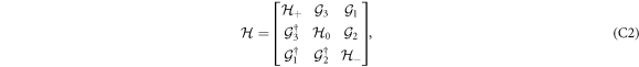
C.1. Diagonal blocks
The diagonal blocks of (C2) are given by (for τ = 0, ±)

Rashba spin–orbit coupling


where 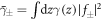 , and have substituted χ = χ+ so that
  , with

with  .
.
Effective mass

Effective ISB parameter—As the ISB value rapidly decays in the second and deeper layers, we assume that it is only finite in the interface layer and zero in the bulk, i.e.  , with a being the lattice constant. In this case, the effective ISB parameter is read as

which can be obtained once the variational parameters are known. In the the weak field regime, by substituting equation (B21) the above can be explicitly expressed as

while in the strong field limit, we have

C.2. Off-diagonal blocks
The off-diagonal blocks of (C2) are given by


where the hybridization parameters are


and


In the above, we have defined the integrals  . Explicitly, they are given as


Appendix D.: Quasi-degenerate perturbation theory
The Hamiltonian (C2) can be decomposed into three subspaces via the Lowdin partitioning [23], i.e.
where the effective Hamiltonian of the each subspace is derived as


Substituting the off-diagonal matrix  into the above, and to the leading order in the ξSO, we obtain the k-cubed corrections as

for  , in which the cubic SOC parameters are derived as


in which  . As the le+ band lie far above the he and le− bands, its corresponding wavefunction is more spreading into the bulk. As a consequence, one can show that
  , and
, and  , so that
  . Therefore, in equations (D6) we retain only the second term,i.e.,
  .
.
In the weak electric field regime, we have following approximations to the leading order in the E-field


where  . The above equations show the dependence of the cubic RSOC on the electric field as
  .
.
Appendix E.: Orbital occupancy
The occupancy of the orbitals in each band can be obtained by representing the eigenstates of the effective Hamiltonian in terms of the t2g basis as

for τ = 0, ±, and i = xy, yz, zx. Then  is referred to as the occupancy of the i-orbital in the τ bands. Around the Γ-point, the occupancies can be analytically obtained as


where  are equivalent to 0, ± bands, respectively. It can be verified that the orbital occupancies satisfy
  for each band.
Substitute χ = χ+ given in (B14), the above expressions reduce to

