


Abstract
Electrons can be energized during laser-driven magnetic reconnection, and the energized electrons form three super-Alfvénic electron jets in the outflow region (Lu et al 2014 New J. Phys. 16 083021). In this paper, by performing two-dimensional particle-in-cell simulations, we find that the electrons can also be significantly energized before magnetic reconnection occurs. When two plasma bubbles with toroidal magnetic fields expand and squeeze each other, the electrons in the magnetic ribbons are energized through betatron acceleration due to the enhancement of the magnetic field, and an electron temperature anisotropy  develops. Meanwhile, some electrons are trapped and bounced repeatedly between the two expanding/approaching bubbles and get energized through a Fermi-like process. The energization before magnetic reconnection is more significant (or important) than that during magnetic reconnection.
Export citation and abstract BibTeX RIS

Content from this work may be used under the terms of the Creative Commons Attribution 3.0 licence. Any further distribution of this work must maintain attribution to the author(s) and the title of the work, journal citation and DOI.
1. Introduction
Magnetic reconnection is a fundamental physical process in plasmas during which the topologies of magnetic field lines are rearranged and magnetic energy is converted to plasma kinetic energy [1–3]. Magnetic reconnection is widely believed to be responsible for various kinds of explosive phenomena in space and laboratory plasmas, such as solar flares [4–6], magnetospheric substorms [7–9], and sawtooth crashes in tokamaks [10, 11]. The generation of energetic electrons is considered to be one of the most important signatures in magnetic reconnection [12–14]. Generally, two-dimensional (2D) particle-in-cell (PIC) simulations show that electrons can be accelerated by the parallel electric field when they move towards the X-line [15–17], and get further accelerated in the vicinity of the X-line by the reconnection electric field [18, 19]. Moreover, Hoshino et al [20] suggest that the electrons can also be accelerated in the magnetic pileup region during the curvature and gradient drift motions after the acceleration in the vicinity of the X-line.
In addition to the above non-adiabatic acceleration mechanisms, adiabatic betatron acceleration and Fermi acceleration are also proposed to explain the generation of energetic electrons in plasmas, especially in geospace and astrophysical plasmas [21–27]. Betatron acceleration works on the magnetized electrons in the enhancing magnetic field. The enhancement of the magnetic field leads to the generation of the inductive electric field, and the magnetized electrons are thus accelerated in the perpendicular direction by the inductive electric field. In contrast, Fermi acceleration is mainly in the parallel direction during which the magnetized electrons gain energy though head-on collision with the magnetic field. The classic Fermi acceleration can also be comprehended through the second adiabatic invariant  taken over a bounce orbit. When the orbit shrinks/contracts, the conservation of
  leads to the increase of
  .
.
Dedicated laboratory experiments have been conducted to study magnetic reconnection, for example, the Todai Spheromak-3 [28, 29], the Swarthmore Spheromak Experiment facility [30, 31], the Magnetic Reconnection Experiment [32, 33], and the Versatile Toroidal Facility [34, 35]. More recently, magnetic reconnection experiments in laser-produced high-energy-density plasmas have also been conducted with the OMEGA laser facility [36, 37] and the Vulcan laser facility at the Rutherford Appleton laboratory [38–40], which provide a new experimental platform to study magnetic reconnection. In the experiments, two (or more) plasma bubbles with high density ( and high temperature (
 are generated by focusing two nanosecond-duration laser beams on a planar-target foil. During the laser-plasma interaction, nonparallel density and temperature gradients lead to the spontaneous formation of azimuthal magnetic fields around the laser focal spots [41]. The azimuthal
  magnetic field is found on the order of megagauss (MG), and forms toroidal ribbons wrapping around the plasma bubbles. When the laser beams are close enough, the bubbles eventually encounter each other with magnetic fields of opposing signs, and magnetic reconnection will occur.
The laser-driven magnetic reconnection experiment has also been conducted to at the Shenguang-II (SG-II) laser facility [42]. Electrons energized up to MeVs are observed in the outflow region of the reconnection experiment, and three well-collimated high-speed electron jets are generated. By performing 2D PIC simulations, Lu et al [43] have investigated the formation of the three high-speed electron jets, which are super-Alfvénic in laser-produced plasma reconnection. During magnetic reconnection, electrons can be accelerated by the reconnection electric field in the vicinity of the X-line. These accelerated electrons move away from the X-line, forming the upper and lower super-Alfvénic electron jets. Meanwhile, electrons can also penetrate into the reconnection pileup region, gyrate in a semi-circle, and get accelerated by the inductive electric field in the pileup region. These accelerated electrons form the center super-Alfvénic electron jet.
In this paper, we further demonstrate that, before magnetic reconnection occurs, the electrons can be energized significantly through betatron and Fermi-like acceleration. The expansion and approach of the plasma bubbles play essential roles in the electron energization processes. The remainder of the paper is organized as follows. Section 2 describes the simulation model, section 3 presents the simulation results, and section 4 gives the summary and discussions.
2. Simulation model
The simulation model used in the present study is a 2D PIC model in which the electromagnetic fields are defined on grids and updated by solving Maxwell equations with a full explicit algorithm. The positions and velocities of the ions and electrons are advanced relativistically in the electromagnetic fields. A first-order weighting is employed for the particle shape factor. The parameters and geometry in the simulations are all in accordance with the SG-II experimental setup [42]. The initial configuration of the simulation system is two expanding semicircular plasma bubbles, similar to the previous PIC simulations by Fox et al [44, 45] and Lu et al [43, 46]. The simulation domain is a rectangular in the  plane with
  and
and  The two semicircular bubbles are centered at
  and
and  respectively. Define the radius vectors from the center of each bubble,
  and
and  .
.
The initial density is  where
where  is the background density, and the density contribution from each bubble
  (
( is
is

Here  is the initial scale of the bubbles and
  is the initial peak bubble density. In the simulation, we choose
  The initial expansion velocity of the bubbles is
  where
where  (
( is
is

and  is the initial expanding speed of the two semi-bubbles. The initial magnetic field is the sum of two toroidal ribbons
  with
with

where  is the magnitude of the initial magnetic field, and
  is the half-width of the magnetic ribbons. To be consistent with the plasma flow, an initial electric field
  is imposed, while the initial current density is determined by Ampere's law.
Table 1 lists the reported or otherwise estimated parameters for the SG-II experiment [42]. Table 2 lists the numerical parameters used in the simulations. The measured electron density near the X-line of reconnection is  which is on the order of one tenth of the peak electron density based on the simulations. The peak electron density is thus about
  Given the average ionic charge
  the peak ion density is about
  Therefore, the ion inertial length based on the peak ion density is
  In the experiment, the radius of the plasma bubbles is about
  and the width of the magnetic ribbons is about
  So in our simulation, we choose
  and
and  As the plasma bubbles expand and squeeze each other, the magnetic field can be enhanced several times compared to the initial value. The enhanced magnetic field is measured to be about
  in the experiment. Thus, we choose the initial magnetic field
  in the simulation. The mass ratio
  and the light speed
  where
where  is the Alfvén speed based on
  and
and  The initial velocity distributions for the ions and electrons are Maxwellian with bulk velocity in the radial direction and drift velocity in the out-of-plane direction. Uniform ion and electron initial temperatures
  are adopted for simplicity. The expansion speed of the plasma bubbles is on the order of the sound speed
  In the simulation, we choose the initial expanding speed
  The cell dimensions are
  with the spatial resolution of
  where
where  is the electron Debye length. Therefore,
  and
and  The time step is
  where
where  is the ion gyrofrequency based on
  About
About  particles per species are employed to simulate the plasmas. Periodic boundary conditions are used in both the
  and
and  directions.
Table 1. Shenguang-II experimental parameters [42].
| Parameter | Reported or estimated values | |
|---|---|---|
| Ions | Al | |
| Average ionic charge |

|
∼10 |
| Peak electron density |

|

|
| Peak ion density |

|

|
| Plasma bubble scale |

|

|
| Width of magnetic ribbon |

|

|
| Temperature |
 
|

|
| Magnetic field |

|

|
| Estimated inflow speed |

|

|
| Ion inertial length |

|

|
| Alfvén speed |

|

|
| Electron beta |

|
2.9 |
| Sound speed |

|

|
Table 2. Simulation parameters.
| Parameter | Simulation setup |
|---|---|

|
100 |

|
0.026 |
![$[{L}_{x}\times {L}_{z}]/{d}_{{\rm{i}}}$](https://content.cld.iop.org/journals/1367-2630/18/1/013051/revision1/njpaa0ba4ieqn85.gif)
|

|

|

|

|
0.05 |

|
0.0001 |

|
12 |

|
2 |

|
75 |

|
3 |

|
0.2 |
Particle number per cell at 
|
500 |
| Total particle number per species |

|
In the simulations, we choose  which is larger than that in some other PIC simulations [27, 47] (nevertheless, it is still much smaller than the realistic value). Our purpose is to pick a small thermal speed in comparison to the speed of light. If the initial thermal speed is comparable to the speed of light, the electrons are thus already relativistic at the initial time, which is far from the realistic experimental setup. In PIC simulations, to accommodate the available computer resources, it is common to use a nonrealistic mass ratio (100 or even smaller), not only in the simulations of the geospace plasmas [27, 47], but also in the simulations of the plasmas in laboratory [45, 48]. The mass ratio
  can distinguish the motions of the electrons and the ions well. The kinetic physics is not sensitive to the mass ratio qualitatively, so the energization mechanisms discussed in this paper do not change with different mass ratios.
3. Simulation results
Figure 1 shows magnetic field lines and contours of the magnetic field  and the portion of the energetic electrons
  (where
  is the local electron density, and the energetic electrons are the electrons whose energy is larger than
  at
at  0, (b) 1.1, and (c) 2.0. Panel (a) gives the initial condition for the magnetic field (equation (3)). At the initial time, the portion of the energetic electrons is very low, about 5%. As the two plasma bubbles expand at a supersonic speed, they strongly squeeze each other, which piles up the magnetic flux in the inflow region before reconnection occurs. At
  just before the beginning of the reconnection, the upstream magnetic field is strongly enhanced, with a maximum of about
  Meanwhile, a long and thin current sheet forms between the two plasma bubbles. The electrons are significantly energized, especially in the magnetic ribbons and the region between the two plasma bubbles. In these regions, nearly 40% of the electrons are energized to
  At
At  two reconnection X-lines generates in the current sheet, and a plasmoid forms between the two X-lines. The portion of the energetic electrons is still high in the reconnection outflow region.

Figure 1. Magnetic field magnitude  (left column) and the portion of the energetic electrons whose energy is larger than
  (right column), at
  0, (b) 1.1, and (c) 2.0. The black curves denote the magnetic field lines in the
  plane.
Download figure:
Standard image High-resolution imageFigure 2 presents the electron (a) parallel temperature  (b) perpendicular temperature
  and (c) temperature anisotropy
  at
at  In the magnetic ribbons, a strong electron temperature anisotropy develops. In the region denoted by the blue box, the electron parallel temperature
  and the perpendicular temperature
  The corresponding temperature anisotropy is thus
  From
From  to 1.1, the electrons are mainly heated in the perpendicular direction. Figure 3(a) shows the velocity distribution of the electrons in the blue box in figure 2. The red arrows denote the directions of the local magnetic field which is mainly along the
  direction. The electron distribution is bi-Maxwellian with the perpendicular temperature higher than the parallel temperature. Figure 3(b) shows the velocity distribution of the accelerated electrons in the red box in figure 2. The velocity distribution is spread out mainly in the
  direction, which indicates that the acceleration in the field reversal region is mainly in the
  direction.

Figure 2. Electron (a) parallel temperature  (b) perpendicular temperature
  and (c) temperature anisotropy
  at
at  The corresponding magnetic field lines are also plotted.
Download figure:
Standard image High-resolution image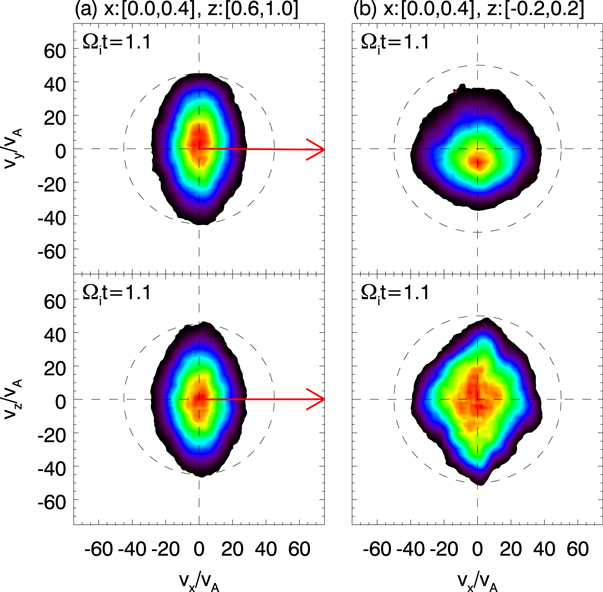
Figure 3. Electron velocity distributions  (top panel) and
  (bottom panel) in (a)
 ![$x\in [\mathrm{0,0.4}]c/{\omega }_{{\rm{pi}}},$](https://content.cld.iop.org/journals/1367-2630/18/1/013051/revision1/njpaa0ba4ieqn130.gif)
![$z\in [\mathrm{0.6,1}]c/{\omega }_{{\rm{pi}}},$](https://content.cld.iop.org/journals/1367-2630/18/1/013051/revision1/njpaa0ba4ieqn131.gif) and (b)
and (b) ![$x\in [\mathrm{0,0.4}]c/{\omega }_{{\rm{pi}}},$](https://content.cld.iop.org/journals/1367-2630/18/1/013051/revision1/njpaa0ba4ieqn132.gif)
![$z\in [-\mathrm{0.2,0.2}]c/{\omega }_{{\rm{pi}}}$](https://content.cld.iop.org/journals/1367-2630/18/1/013051/revision1/njpaa0ba4ieqn133.gif) at
at  The two regions are marked by blue and red rectangles, respectively, in figure 2. The red arrows denote the direction of the local magnetic field, and the dashed circles represent the isotropic distributions.
Download figure:
Standard image High-resolution imageTo further investigate the electron energization mechanism in the magnetic ribbons, we 'tag' the electrons in the blue box (see figure 2) at  and re-run the simulation to trace the positions and energies of the tagged electrons. Figure 4 presents the spatial and energy distributions of these tagged electrons at three different times,
  0, (b) 0.5, and (c) 1.0. Initially, most of the electrons are located in the magnetic ribbons with the energy around the initial temperature
  At
At  the electrons are energized, with the average energy of about
  The average energy is further enhanced to about
  at
at  and some of the electrons can be accelerated to higher energy, over
  Note that the electron energization is accompanied by the magnetic field enhancement, and most of the energized electrons are magnetized in the magnetic ribbons, which suggest a process of betatron acceleration.

Figure 4. Positions of electrons are traced backward in time at  0, (b) 0.5, and (c) 1.0. The electrons are located in the blue rectangle in figure 2 at
  The colors of the dots represent the kinetic energies
  for each electron. The plots are zoomed in on the upper plasma bubble to show the colored particles more clearly.
Download figure:
Standard image High-resolution imageA representative electron, electron 1, is presented in figure 5 to further illustrate the electron betatron acceleration process in the compressed magnetic ribbons. Figures 5(a)–(c) show the trajectory of the electron during different time intervals. The background contours show the magnitude of the magnetic field, and the magnetic field lines are also plotted for reference. Figures 5(d) and (e) plot the time evolutions of the electron kinetic energy  and magnetic moment
  respectively. It is easy to note that the electron is magnetized in the ribbons all the time from
  to 1.1, during which the magnetic field is enhanced from
  to nearly
  The electron is accelerated from about
  to about
  and the magnetic momentum of the electron is almost kept as a constant,
  The enhancement of the magnetic field leads to the generation of the inductive electric field in the magnetic ribbons, and the magnetized electrons are accelerated in the perpendicular direction by the inductive electric field. Therefore, electron 1 is energized through betatron acceleration, and this kind of energized electrons forms a bi-Maxwellian distribution with the electron temperature anisotropy (
 see figure 3(a)).
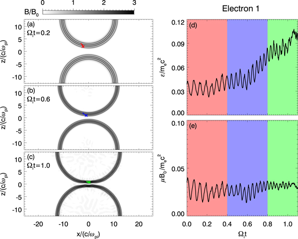
Figure 5. A representative betatron accelerated electron, electron 1. Panels (a)–(c) show the trajectory of electron 1 during (a)  (b)
(b)  and (c)
  The background images are the magnetic field magnitude
  at
at  0.2, (b) 0.6, and (c) 1.0. Panels (d) and (e) plot the time evolutions of the electron kinetic energy
  and magnetic momentum
  respectively.
Download figure:
Standard image High-resolution imageIn the magnetic field reversal region between the two expanding bubbles, the electrons can also be energized significantly, especially in the  direction (see figure 3(b)). We also trace the trajectories and energies of all the electrons in the red box (see figure 2) at
  Figure 6 shows the positions and energies of these electrons at
  0, (b) 0.5, and (c) 1.0. The electrons are initially located in the region outside of the plasma bubbles, namely the background region, with an averaged energy of about
  As the expansion and compression of the two plasma bubbles, the electrons are accelerated at the edges of the magnetic ribbons. The averaged energy of the tagged electrons increases to about
  at
at  and over
  at
at  Some of the electrons can be accelerated to relativistic energy, over
  Figures 7(a)–(c) show the orbit of a representative energetic electron, electron 2, for the time interval from
  to 1.1. Figures 7(d) and (e) show the time evolutions of the kinetic energy and velocity of the electron respectively. The electron moves in the background region and bounces repeatedly between the two expanding bubbles. From
  to 1.1, electron 2 is reflected sixteen times between the two plasma bubbles (or magnetic ribbons) in the
  direction. During each of the reflections, the electron gains a larger absolute value of
  At the same time, the electron is accelerated in the
  direction by the inductive electric field
  where
where  is the radial expansion speed and
  is the toroidal magnetic field. As the accumulation of this kind reflection, electron 2 is accelerated with the energy increases from about
  to about
  Figure 8 further shows the kinetic energy of electron 2 as a function of its
  position. The electron gains energy as it is reflected by magnetic ribbons at the boundaries of the bubbles, which suggests that the energization process of electron 2 is a Fermi-like process.

Figure 6. Backtrace of the electrons located in the red rectangle in figure 2 at  Same format as figure 4.
Download figure:
Standard image High-resolution image
Figure 7. A representative Fermi-like accelerated electron, electron 2. Panels (a)–(c) show the trajectory of electron 2 during (a)  (b)
(b)  and (c)
  The background images are the magnetic field magnitude
  at
at  0.2, (b) 0.6, and (c) 1.0. Panels (d) and (e) plot the time evolutions of the electron kinetic energy
  and velocity components
 and
and  respectively.
Download figure:
Standard image High-resolution image
Figure 8. Kinetic energy of electron 2 as a function of its  position.
Download figure:
Standard image High-resolution imageThe magnetic field shows a wavy structure along the toroidal direction (parallel to the magnetic field) of the compressed magnetic ribbons. Figure 9 depicts the zoomed-in structures of the magnetic field lines and the out-of-plane magnetic field  at
at  0.65, (b) 0.9, and (c) 1.8. At
 shows a wavy structure with alternate positive and negative values along the direction parallel to the magnetic field. The wavelength of the structure is about
  The wavy magnetic field perturbation grows stronger at
  (see figure 9(b)). Besides the out-of-plane magnetic field
  the in-plane magnetic field (indicated by the magnetic field lines) is also wavy. At
  due to the Hall effect of magnetic reconnection, there forms the quadrupolar structure of
  During the same time, the wavy magnetic field perturbation gradually decreases. At the edges of the magnetic ribbons, the magnetic field is weak and the electron temperature is anisotropic, which is favorable to the Weibel instability [49]. The wavy magnetic structure along the parallel direction is considered to be the consequence of the Weibel instability.
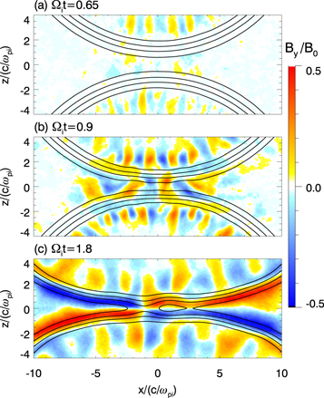
Figure 9. Out-of-plane magnetic field  at
at  0.65, (b) 0.9, and (c) 1.8. The black curves denote the in-plane magnetic field lines.
Download figure:
Standard image High-resolution imageFigure 10 depicts the time evolution of  perturbation at the inner edge of the magnetic ribbons. After about
  the wavy
  grows up from the noises, and keeps growing until about
  after which the
  perturbation begins to saturate. The red dashed line shows an exponential fit to the growth stage,
 ![${B}_{y}~\mathrm{exp}[{\gamma }_{{\rm{sim}}}(t-{t}_{0})],$](https://content.cld.iop.org/journals/1367-2630/18/1/013051/revision1/njpaa0ba4ieqn209.gif) with the fitted growth rate
with the fitted growth rate  and
and  is the time when the wavy perturbation begins to grow. Based on the analytical theory [50], the Weibel instability occurs for wavelengths such that


Figure 10. Time evolution of the magnetic field wavy perturbation  At each time step, the amplitude of the wavy perturbation is defined as the maximum value of
  in the region
 or
or  The gray area indicates the linear growth phase, and the dashed line shows an exponential fit, with the fitted growth rate obtained from the simulation
  .
.
Download figure:
Standard image High-resolution imageThe growth rate reaches its maximum at  with
with

where  is the electron plasma frequency. For


 and
and  as measured at the inner edge of the magnetic ribbons where the instability is excited at
  based on the above analytical theory, the maximum growth rate is estimated as
  and the wave number
  corresponding to the wavelength
  The wavelength obtained in the simulation is found to be consistent with the analytical theory, and the growth rate
  is also close to the analytical
  The above consistency between the simulation and linear theory shows that the formation of the wavy
  perturbation is due to the Weibel instability driven by the electron temperature anisotropy.
After about  magnetic reconnection begins, and the electrons are further energized. Figure 11 shows the contour of the electron bulk velocity
  at
at  and two representative electrons (electrons 3 and 4) that are accelerated during the reconnection process. At
  electron 3 has been accelerated to about
  through betatron acceleration in the magnetic ribbons. In the vicinity of the X-line (or electron diffusion region), the magnetic field is weak. The electron moves towards the X-line due to the magnetic mirror force
  Once the electron moves into the electron diffusion region, the electron is accelerated by the reconnection electric field
  therein from
  to
to  After
After  the accelerated electron 3 then leaves the X-line along magnetic field lines. Background electrons can also be accelerated in the magnetic pileup region of the reconnection. During
  a background electron (electron 4) moves towards the reconnection pileup region with a relatively lower energy. The magnetic field in the background region is very weak, so there is a sharp boundary between the background region and the pileup region. At about
  the electron penetrates through the boundary and moves into the pileup region. In the pileup region, it senses a
  Lorentz force, which causes it to gyrate for about half an orbit. At the same time, the electron is accelerated in the
  direction by the inductive electric field
  in the pileup region. At about
  after the semi-cycle, the electron leaves the pileup region and moves back into the background region along the
  direction with a higher energy of about
  .
.

Figure 11. (a) Electron bulk velocity in the  direction
  at
at  and trajectories of electrons 3 (green) and 4 (red) during
  and
and  respectively. Panels (b) and (c) plot the time evolutions of the kinetic energy
  of electon 3 and electron 4 respectively.
Download figure:
Standard image High-resolution imageFigure 12 plots the electron energy spectra in the whole simulation domain at  1.1, and 2.0. At the initial time, the electron distribution is Maxwellian with a temperature of about
  At
At  just before the reconnection begins, the electrons are strongly heated/accelerated through betatron and Fermi-like processes, with the high energy part extends beyond
  After the beginning of magnetic reconnection, at
  the electrons are further energized by the reconnection process. Note that the energization through betatron and Fermi-like processes before magnetic reconnection is more significant than the energization by magnetic reconnection.

Figure 12. Electron energy spectrum computed in the whole simulation domain at  1.1, and 2.0.
Download figure:
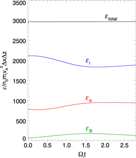
Standard image High-resolution imageTime evolutions of total energy  ion kinetic energy
  electron kinetic energy
  and magnetic energy
  are shown in figure 13. It is noted that the total energy is well conserved in the simulations. Based on the energy evolutions, the whole process of the laser-driven reconnection can be summarized as follows: the initial supersonic expansion of the plasma bubbles leads to the enhancement of the magnetic field, and the electrons are energized through betatron and Fermi-like processes. Therefore, at the early stage, the ion kinetic energy is converted to the magnetic energy and electron kinetic energy. At the second stage after magnetic reconnection begins, the increase of the magnetic energy slows down due to the dissipation caused by reconnection. At the last stage, the expansion of the bubbles is gradually stopped, reconnection becomes the dominant process. The magnetic energy is converted to the kinetic energies of the electrons and ions through magnetic reconnection.
Figure 13. Time evolutions of total energy  ion and electron kinetic energies
 and magnetic energy
  The total energy
  Here
Here  is the energy of the electric field which is very small and thus negligible.
Download figure:
Standard image High-resolution image
4. Conclusions and discussion
In this paper, based on the geometry and parameters of the SG-II reconnection experiment, we performed 2D PIC simulations to investigate the electron energization in laser-driven magnetic reconnection. The electrons were found to be energized to high energy before magnetic reconnection occurs, and the following magnetic reconnection can further energize these electrons. The energization before magnetic reconnection is more significant than that during magnetic reconnection. Before magnetic reconnection occurs, the magnetic field of the magnetic ribbons is enhanced due to the expansion of the plasma bubbles and the compression between the bubbles, which leads to the betatron acceleration of the electrons therein. The betatron acceleration is mainly in the perpendicular direction, therefore, an electron temperature anisotropy  develops. The Weibel instability is excited by the electron temperature anisotropy, which generates a wavy magnetic structure at the edges of the magnetic ribbons. At the same time, some electrons can be bounced repeatedly between the two expanding bubbles and get energized through a Fermi-like process. After magnetic reconnection begins, the electrons are further energized. Part of the electrons can be accelerated by reconnection electric field in the vicinity of the X-line, and then move away from the X-line. Electrons can also be accelerated in the pileup region where they gyrate in a semi-circle, and then leave. During the semi-circle gyration, these electrons are accelerated by the inductive electric field in the pileup region.
The Weibel instability (or filamentation instability) has been found to play an important role in the hot, dense plasmas produced by high-intensity ( picosecond- or femtosecond-duration laser pulses [51–53]. The development of the counter-streaming Weibel instability leads to the generation of the turbulent magnetic fields in the plasmas. On the other hand, in laser-driven magnetic reconnection experiments, the laser beams are nanosecond-duration, and their intensity is
  In the nanosecond-pulse regime, we have demonstrated that the Weibel instability also develops due to the electron temperature anisotropy. Therefore, a turbulent/wavy magnetic structure is also generated at the edges of the magnetic ribbons. The turbulent/wavy magnetic structure may have a significant effect on the reconnection onset.
Magnetic reconnection between laser-produced plasma bubbles is found to be in a strongly driven reconnection regime. Fox et al [44, 45] have demonstrated that the upstream magnetic flux pileup plays an essential role in the sharply increase of the reconnection rate in the laser-driven magnetic reconnection. In the present study, we have further shown that the magnetic flux pileup is also very important for the electron energization. Before magnetic reconnection begins, the upstream electrons are pre-energized through betatron acceleration. These pre-energized electrons are easier to get further energized during magnetic reconnection [16]. As the two expanding plasma bubbles approach to and squeeze each other, a thin current sheet forms between them [46]. The electrons in the current sheet can also be pre-energized by reflections between the two bubbles, which is a Fermi-like process. Therefore, the current sheet is thermalized, corresponding to a high-beta magnetic reconnection which has a low efficiency at converting magnetic energy into the electron kinetic energy [54]. This is why the electron energization by magnetic reconnection is less significant than the enegization by the magnetic flux pileup and plasma bubble expansion.
Acknowledgments
This work was supported by 973 Program (2013CBA01503, 2012CB825602), the National Science Foundation of China, Grant Nos. 41474125, 41331067, 11235009, 41174124, 41274144, 41121003, CAS Key Research Program KZZD-EW-01-4, and the Specialized Research Fund for State Key Laboratories of China.