


Abstract
Financial crises appear throughout human history. While there are many schools of thought on what the actual causes of such crises are, it has been suggested that the creation of credit money might be a source of financial instability. We discuss how the credit mechanism in a system of fractional reserve banking leads to non-local transfers of purchasing power that also affect non-involved agents. To overcome this issue, we impose the local symmetry of time homogeneity on the monetary system. A bi-currency system of non-bank assets (money) and bank assets (antimoney) is considered. A payment is either made by passing on money or by receiving antimoney. As a result, a free floating exchange rate between non-bank assets and bank assets is established. Credit creation is replaced by the simultaneous transfer of money and antimoney at a negotiated exchange rate. This is in contrast to traditional discussions of full reserve banking, which stalls creditary lending. With money and antimoney, the problem of credit crunches is mitigated while a full time symmetry of the monetary system is maintained. As a test environment for such a monetary system, we discuss an economy of random transfers. Random transfers are a strong criterion to probe the stability of monetary systems. The analysis using statistical physics provides analytical solutions and confirms that a money–antimoney system could be functional. Equally important to the probing of the stability of such a monetary system is the question of how to implement the credit default dynamics. This issue remains open.
Export citation and abstract BibTeX RIS

Content from this work may be used under the terms of the Creative Commons Attribution 3.0 licence. Any further distribution of this work must maintain attribution to the author(s) and the title of the work, journal citation and DOI.
GENERAL SCIENTIFIC SUMMARY Introduction and background. We analyze a monetary system of money and antimoney which becomes possible with the advent of computer cryptography. The approach is motivated by the non-local effects of credit creation: a local payment through the creation of credit triggers an inflation that affects all other market participants. Products are bought by credit creation at price levels before the inflationary effects. In the last five years, everyone suffered from local mediocre credit creation between a small number of market participants.
Main results. We borrow structures from the physics of energy and momentum conservation, inspired by the Noether theorems of time homogeneity. Instead of relying on interest rates where local partners judge the future value of past investments for finite time spans, a local exchange rate compares values of the past (debt = antimoney) with values of the future (money). This judgment is performed in real time by all participants in any monetary transaction. The proposed money and antimoney units already exist in banking bookkeeping, but are not treated as separate units: money consists of bank liabilities and non-bank assets while antimoney is memorized as bank assets and non-bank liabilities. Both units are indeed never added or subtracted. Instead of creating credit by new money and debt units, liquidity is transferred by the concurrent transfer of money and antimoney. The exchange rate between both plays the role of interest rates in the contemporary system. To make money non-local, both units have to be normalized to the number of subjects in an economic space. Lacking experiments in economy, we study the monetary structure for random transfers. This has proved to be a crucial stability test for monetary systems.
Wider implications. Clearly, an electronic system has to guarantee that the antimoney units do not vanish, something that was not possible without electronic payment systems. Also, similar to contemporary structures, money insurance schemes have to distribute the risk of subjects leaving the normalized economic space.
 Figure. A direct monetary transfer does not affect the wealth of all other market participants (top). However, if the transfer is performed with a transfer by credit creation, the resulting inflation changes the wealth of the other market participants (bottom). This is the main motivation for creating and discussing a novel monetary structure without localized effects.
1. Overview
The main function of money is to store information on transactions in the economy and to establish a unit of account in the credit–debit record keeping of the banking system [1, 2]. The symmetry properties of this economic memory are important because they entail the local conservation laws that are postulated in much of the literature on monetary theory and the statistical mechanics of money [3]. If a monetary space is not homogeneous in time, the money supply is not fixed, and non-local, unwarranted transfers occur. Consequently, precise storage of economic information is no longer guaranteed. Although these non-local interactions are known in economics as inflation tax, their microscopic effects have largely gone unnoticed in economics and econophysics: the mechanism by which transactions are recorded has economic consequences for all agents. Since the money supply in real world economies is largely driven by demand for credit, contemporary monetary systems systematically violate time homogeneity and consequently are rather imperfect stores of economic information [2].
The statistical mechanics approach has proven highly successful in determining the global properties of monetary systems subject to different boundary conditions [3–9]. All of this work however contains the local conservation of money as a postulate and deals only with nominal money, ignoring the effective redistributive taxation that comes with the creation and annihilation of monetary units. In economics, the Friedman rule holds that a constant money supply improves welfare, however the problem of liquidity shortages under such a regime has not been resolved [10].
Symmetries of monetary spaces are therefore of high interest both in econophysics, because symmetries restrict system behavior, as well as economics, because such restrictions potentially lead to unnecessary inflexibility. But a monetary system that is homogeneous in time would be beneficial because it would keep the money supply constant. In the following we show how invariance under time translation and exchange of trading roles leads to conserved quantities and present a fully symmetric toy model of a monetary system that addresses the problem of liquidity shortages through a new type of monetary transfer.
Lacking the ability to conduct economic experiments, we then study this new economic structure under the assumption of random transfers. Under random transfer, the stability of economic structures can be crucially tested as the random walk tends to create inflationary scenarios in creditary monetary systems [7, 11]. We can derive a number of analytical solutions for such a time symmetric monetary system for the case of random transfers.
2. Background
The origin of money and even a correct definition of money are still subject to debate [12, 13]. Most economic textbooks today define money by its functions. ('Money is what money does' [14].) It is useful to distinguish between commodity money and representative money. Commodity money fulfills the aforementioned criteria because of a perceived intrinsic value of the material it is made of, such as gold or silver. Representative money on the other hand is essentially a claim on goods or services to be rendered in the future. This function heavily depends on social and legal measures to enforce these claims. Being a social contract, it is independent of its physical representation, best seen in electronic payment systems. Historically, representative money is inextricably linked to the record of debt relations [15, 16]. If a buyer wasn't able to pay for a good immediately, the seller could grant him a credit if he had sufficient trust in the economic potential of the buyer. They would record their debt relation for example by the use of tally sticks or clay tablets [17] (see figure 1).

Figure 1. Two examples for records of debt relations which served as currencies. (a) Tally sticks were commonly used in medieval Europe. A marked wooden stick representing the transactional value was split into halves of different lengths. The creditor kept the longer part (stock) and the debtor was given the shorter one (foil). The stock represented a claim to future income and was actively traded (stock market). In contrast to commodity money, the creation of representative money comes at virtually no cost. (b) Clay tablets served a similar function and recorded credit money contracts.
Download figure:
Standard image High-resolution imageIf the debtor was a highly visible agent with a good economic standing, they could serve as a currency [18]. But incomplete information about the market participants and the overhead of enforcing the claims prohibited the wide circulation of these promissory notes. It is often not necessary for the issuer to be able to meet all his obligations at all times [19]. Most of the creditors will then continue to use the notes in trades as they are confident that they could cash the notes at all times if they so desired. The issuer can now create new money by accommodating loans: he can hand out additional promissory notes to a borrower. This service is nowadays provided by commercial banks. The money in a commercial bank account is legally a claim on central bank money which in most countries is fiat money, i.e. money that has been declared legal tender by government decree. The majority of financial transactions today are carried out by commercial bank money. However, if the trust to accept the bank's 'promissory notes' is lacking, bank runs might occur. The bank will have problems finding creditors on the interbank lending market.
One problem with the creation of money via loans is the possible devaluation of the currency [20]. As discussed later, credit creation creates non-local transfers of purchasing power which adversely affect net asset holders. Starting from this observation, we will propose a monetary system of money and antimoney that remedies this deficiency and introduce a novel mechanism for obtaining liquidity.
3. Credit creates non-local transfers of purchasing power
Consider a simplified economy of N + 1 agents where the (N + 1)th agent has gathered sufficient trust in that the other N agents are willing to accept its promissory notes as means of payments. We will call this agent 'bank'. For simplicity, the bank's promissory notes are the only currency in circulation. For our analysis the terms 'promissory notes' and 'demand deposits' are used interchangeably since both represent a client's claim to an underlying entity that the bank promises to meet.
Every agent keeps a so-called T-account to record his assets in the left column and his liabilities in the right column (cf figure 2). The agents' assets are liabilities of the bank and vice versa. The assets and liabilities that agent k holds at time  are denoted
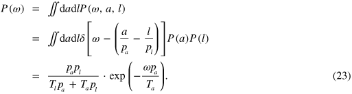
  and
and  . The total monetary supply at time
  is
is

Electronic bookkeeping shall prevent monetary units from being lost or destroyed. If agent i buys some good from agent j and they have agreed on a price  , then agent i has several payment options. He can directly transfer the amount
  from his asset account to j's asset account. When the trade happened between
  and
and  and no other transactions occurred in that time period, the asset holdings after the trade will be
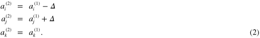
The agents  are not involved in the trade. The liabilities are not affected. Figure 2(a) shows the corresponding bookkeeping operation. The total money supply hasn't changed:
  . If we look at the relative monetary wealth of the total monetary supply that each agent holds

we see that the relative monetary wealth of the agents k remains unaffected:

This is not the case if i chooses to pay by credit creation (cf figure 2(b)):
Now, the total money supply used in trades has increased:  . We see that the relative monetary wealth of non-involved agents k after the trade has changed: if we now look at

the shift in relative asset and liabilities holdings is given by
Thus, we see that credit creation is potentially beneficial for all debtors and adversely affects all creditors (figure 3). Only in the case of  , non-involved agents are unaffected by credit creation. Indeed, since
  , we see that there is an indirect transfer of relative monetary wealth from creditors to debtors.

Figure 2. All monetary transactions can be visualized in a T-account. Here, only the updates in the balance sheets are shown. Figure (a) shows a direct transfer of asset units from buyer i to seller j. A payment via credit creation (b) leads to an increased money supply and—as will be shown later—to non-local transfers of purchasing power. The reverse process of credit annihilation (c) occurs when a creditor pays a debtor and leads to a decrease of the total money supply. Note, of course, that credit annihilation can only occur after credit creation.
Download figure:
Standard image High-resolution image
Figure 3. The shift  of relative asset and liability holdings that non-involved agents experience when a trade is executed either by direct asset transfer or by credit creation. Note that in the case of a direct transfer, non-involved agents experience no change at all. In the case of credit creation, the agents' relative share of assets and liabilities decreases and thus agents with
  are at a disadvantage according to equation (7). Conversely, if
  , agents profit from credit creation. It is only when agents hold the same amount of assets and liabilities, that they are unaffected by credit creation.
Download figure:
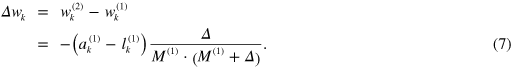
Standard image High-resolution imageIn the case of credit annihilation (see figure 2(c)), the reverse effect occurs. As the total money supply decreases, the sign in equation (7) is reversed. One might conjecture that both effects somehow cancel. But it has been shown that unrestricted fractional reserve banking leads to an increase of the money supply without bounds [7]. This is due to the fact that the number of loans (which create asset–liability pairs) cannot be negative. In reality, bank lending is not completely unrestricted but nevertheless a net increase of credit is confirmed by virtually all statistics about the money supply M1 [21].
Let us assume that agent k knows that the trade between i and j happened by credit creation and that the transferred amount of money was  . If k previously charged a price
  for his services, he might now set a new price
  to compensate for his loss of relative monetary wealth. From the condition

we find that the expected new price should be

which is obviously larger than  . Note that
  with N being the total number of market participants. Since the price change
  is a detailed function of asset
  and liability holdings
  , there is no global factor by which agents k could rescale their prices in order to get back to their initial situation. A non-local transfer of wealth is the result. The reaction of agents to inflation expectations assumes a widespread knowledge about credit creation processes. Credit creation—ceteris paribus—leads to increasing price levels. In a real economy, those agents who are 'closest' to the credit creation profit the most from it as they will still face the old prices. This effect has already been described by Richard Cantillon in the 18th century and has subsequently been named the Cantillon effect [22].
Of course, credit creation is not the only source of inflation. Inflation—especially in the short run—depends on several factors including but not limited to money supply, technological advancement, real demand, production and stability of governments. Most economists believe an extension of the money supply to be the prime cause for inflation in the long term [23]. The question of the particular benefits and disadvantages of inflation is an ongoing debate. In most countries, general price stability has become one of the major goals of monetary and fiscal policies [24–26] and in some even the most predominant one [26]. Inflation, whether it be anticipated or unanticipated, is costly for society due to deadweight losses [27]. For small inflation rates (around 2%), most economists have come to consider the negative consequences being outweighed by a range of positive effects [28–31]. These include an increased maneuverability of central banks near the zero lower bound of nominal interest rates and the ability for firms to counteract the downward rigidity of nominal wages. As deflation is often considered even worse than inflation, a small rate of inflation can also serve as a buffer. A recent working paper of the International Monetary Fund suggests that the corridor of acceptable inflation rates might be narrower than previously thought [32]. The issue of money-induced inflation has of course been recognized and debated, e.g. in connection with the bank charter act of 1844 which prohibited commercial banks from issuing promissory notes [19] and by several other authors [20, 33–38].
4. A time-homogeneous bi-currency system of money and antimoney
In order to prevent non-local transfers upon credit creation and to attenuate the Cantillon effect, the usually proposed solutions essentially restrict credit creation by commercial banks or prohibit it entirely [39–42]. These proposals have come to be known as narrow banking, full reserve banking or 100% reserve banking. A very strict implementation of full reserve banking has long been dismissed by mainstream economists, but in view of the current financial crises, the idea has gained some traction again [43, 44]. The main criticism of full reserve banking is its alleged inability to provide an economy with the necessary liquidity, i.e. even agents whose creditworthiness is ensured, cannot easily obtain means of payment for future investments [45, 46].
We have seen (figure 2) that representative money always consists of an asset–liability pair: the asset part is the actual claim to a good or a service to be rendered in the future and the liability part is the obligation of the debtor to provide it. Our main idea for a symmetric monetary system is to fully separate both parts by using two monies of equal supply and circulating the agent's asset units independently of the agent's liability units. The respective complementary liability and asset parts are kept at a central bank.
In an analogy to physics, the asset units can be considered as money whereas liability units are antimoney [11, 47]. The analogy is limited in this discussion since money and antimoney do not annihilate and will only be created if agents enter or destroyed if agents leave the economy. Demand deposits at commercial banks are to be fully backed by central bank money, i.e. commercial banks would be prohibited from credit creation. Of course, time and investment deposits could still be fractionally backed. In order to be able to adapt the money supply to economic growth, the central bank would be allowed to directly regulate the amount of money in circulation.
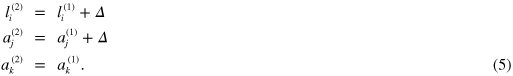
Now agent i can either purchase some good from agent j by transfering  asset units to him or by receiving
  liability units along with the good. To put it briefly, in order for agents to increase their monetary wealth, they want to obtain asset units and get rid of liability units. The feasibility and pitfalls of such a system will be discussed in section 9. Of course,
  and
and  do not have to be accounted for in the same unit. The introduction of antimoney allows the market to continuously assess the value of assets and liabilities and to establish two different nominal price levels
  and
and  for both payment modes. As with any two currencies, this gives rise to a free floating exchange rate between both monies that is missing in the present system. Let us define the equilibrium exchange rate as
  and the implicit exchange rate in a trade as
  . Real monetary wealth in a symmetric monetary system is given by

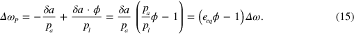
where a and l denote the asset and liability holdings. This is the linear extension to the definition of real purchasing power in economic textbooks [13]. Now if a transfer is executed by either of the two payment options and  , the monetary wealth of the payee changes by

If the seller offers both payment options but asks for prices such that  , he is asking for a premium for one of the payment options. For example he might ask for a premium if the buyer 'pays in liabilities' (i.e. if the buyer agrees to receive liability units):

In addition to the new payment option via liabilities there is now a novel, interesting way to provide liquidity to an agent by simultaneously transferring asset and liability units to him. Assume for a moment that both price levels are equal:  . Then an agent can transfer
  asset and liability units to a liquidity-seeking market participant without changing his monetary wealth. Thus, in a symmetric monetary system as outlined above, monetary wealth and liquidity become different notions, as illustrated in figure 4.

Figure 4. The liquidity of an agent can be limited by either (a) its asset or (b) its liability holdings. The blue line indicates the amount of money and antimoney that would be transferred at a liquidity price  . Here we have assumed
  , i.e. a liquidity provider P would choose to transfer more liability units than asset units. His profit then depends on the equilibrium exchange rate
  .
.
Download figure:
Standard image High-resolution imageLet us turn again to the general case of arbitrary  and
and  . If a liquidity provider P simultaneously transfers
  asset units and
  liability units, his monetary wealth changes by

If he wants to be remunerated for his services, he will set a nominal price of liquidity

such that  . Assume for example an investor who requires means of payments equivalent to a wealth
  . Then the provider's wealth changes by
Thus, in order to profit from the provision of liquidity, the provider should ask for a price  . The formal definition of liquidity of an agent i can then be stated as

How could such a concept help to overcome the issue of credit crunches commonly associated with full reserve banking systems? In a conventional system with 100% reserve requirements, a borrower has to find someone who is actually willing to part with his money for a certain time. This is not the case in a fractional reserve banking system in which the commercial bank can accommodate the loan. In a system of money and antimoney, a buyer would be able to accept antimoney instead of paying with money. Thus, if he wasn't able to find the necessary 'money funds', a trade could still succeed if the seller—not the buyer—had sufficient antimoney.
Another advantage lies in the nature of the liquidity market. In contrast to a system where liquidity is provided by additional loan contracts, the price of liquidity is set at the moment of transfer. In a conventional monetary system the price is determined by the payment of interest, often fixed for a long time span, which carries with it the need for supervision and enforcing the contractual agreements. Thus the legal overhead including time delays is non-negligible for a single agent. In a symmetric monetary system, however, the provision of liquidity is as simple as an ordinary act of purchase.
5. Symmetry considerations
Physical laws of motion are symmetric by nature and governed by the action principle. On the other hand, bookkeeping is a memory of economic transfers, not a physical model of their dynamics. The properties of economic exchange may influence the dynamics of the real economy and are subject to social choice. We will discuss whether the rules of exchange are invariant under certain transformations. As expected from the physical Noether theorem, also economic transaction rules imply conservation laws if they obey certain symmetries. As we will see, the stability of the unit of account and the elimination of non-local transfers is linked to the time homogeneity of a monetary system. Notably, this finding does not imply an action principle in bookkeeping, i.e. a close analogy between mechanics and the nature of economic transactions.
The conservation of either the asset units or the liability units in a transfer is guaranteed by the realization principle. It expresses value conservation by stating that revenue—a gain in assets or loss in liabilities—should only be recognized when an enforceable claim against another party exists to receive the revenue [48]. The realization principle is a consequence of symmetry under exchange of trading roles. Let

denote the account balance of agent i before (t = 1) and after (t = 2) the transfer. The claim is that p is conserved if the transfer is invariant under an exchange of transfer roles, that is, under index permutation  . Let's write a transfer from
  as
as

This does not say anything about conservation yet; it may well be that  and hence
  . Applying
  to both sides gives
  . The sum
  has obviously not changed; the left hand sides however are only equal if
  and hence only if
  is conserved. Note that it is not necessary for either i or j to actually hold
  : as long as
  , the total
  is conserved. It is important to understand that this does not prohibit the creation of new asset–liability pairs, e.g. by the creation of credit.
The conservation of the total amount of monetary units, i.e. either the sum of all assets or the sum of all liabilities is not ensured by a principle in bookkeeping. This indicates that time homogeneity can be systematically violated in bookkeeping. As we saw in figure 3, this leads to problems when new monetary units are created.
Assume two agents hold  at t. We shift the system—the holdings
  —by
—by  :
:  and
and  . If there is no transfer in
  , the derivatives are zero; otherwise

and time homogeneity  is ensured if

which expresses conservation of asset units across time and transfers. An equivalent expression can be derived for liability accounts  . If the quantity of money—either the asset units
  or the liability units
  —is not conserved, new money can be created during transfer. Due to momentum conservation it is created as a pair and we find
  . A corollary of equation (20) is that the payer needs to get hold of the assets before the transfer. Since
 , we have
  for all transfers
  from
from  . Thus some transfers fail only because liquidity is lacking. Under time homogeneity, a stricter order of transfers is enforced as liquidity has to be obtained from other agents before the transfer.
6. Time-homogeneous money in random economies
In order to make predictions about economic quantities in a monetary system, we need a model that describes the interactions between market participants. As human behavior is notoriously hard, if not impossible, to capture in models, a growing amount of research in this field has focused on random economies in which agents exchange random amounts of money, much like particles exchange energy [3, 7–9]. This reflects the fact that the environment of an economy and the future of investments are hard to predict also for the agents—in the extreme case the environment can be considered fully random. Surprisingly, such an economic null model correctly predicts monetary wealth distributions for all but the richest subpopulation [3]. Moreover, it is a challenging test bed to probe the stability of monetary systems [7, 49].
We study the time-homogeneous monetary system proposed in the previous section with the model of a random economy. Agents exchange random amounts  of asset and liability units drawn from an exponential price distribution

where  and
and  is the respective price level. That particular choice is motivated by private observations [11] which confirm that in real economies transfers with low prices are encountered much more often than high prices. However, the distribution of transfer prices is not critical to the outcome: Dragulescu and Yakovenko have shown that the equilibrium monetary distribution in a closed single currency system is given by a Boltzmann–Gibbs distribution for a wide range of random transfer schemes, namely those that have time-reversal symmetry [9]. If we consider the money and antimoney holdings to be independent of each other (i.e. if we disregard the liquidity providing mechanism introduced in the previous section), we should expect both distributions to equilibrate to Boltzmann–Gibbs distributions as well:
where  . The parameter
  , with
  being the total amount of asset or liability units and N being the number of market participants, is equivalent to a temperature in statistical physics. The corresponding simulation in figure 5(a) confirms this expectation. In contrast to a single currency economy, the wealth distribution is now distinct from the money distribution. Let
  be the probability of finding an agent with wealth
  , a assets and l liabilities. Considering that the probability distributions of a and l are only well-defined for positive values, the marginal probability of finding an agent with wealth
  is:
is:
For negative values of  one finds

So we see that the wealth in a symmetric monetary system with a random economy is distributed according to a Laplace distribution (see also figure 5(b)). Interestingly, this distribution is very similar to the one found in a system with fractional reserve banking [8]. This is to be expected since both models impose a cap on global dept by limiting the total number of asset–liability pairs. The first moment of the wealth is given by
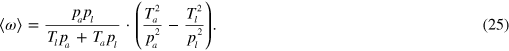

Figure 5. Money and wealth distributions with (c), (d) and without (a), (b) a liquidity market (LM). (a) In a random economy without liquidity transfer, asset and liability holdings both equilibrate to a Boltzmann–Gibbs distribution. (b) According to equation (23), the monetary wealth distribution also depends on the price levels  and
and  and may thus be asymmetric. The black lines in (b) were calculated using equations (23) and 24) whereas points represent random transfer simulations with N = 100 000 agents. (c), (d) Simulation results with a LM. (c) Except for two outliers with no assets or liabilities, the distribution of assets and liabilities still largely follows an exponential law with effective temperatures
  . (d) If a liquidity market is present (shown for
  and
and  ), the resulting wealth distribution is broader than in the case of no liquidity trading. With large
  , the wealth distribution becomes increasingly asymmetric. For simplicity, the simulation was performed using
  and
and  .
.
Download figure:
Standard image High-resolution imageIn order to prevent agents from accumulating an unlimited amount of antimoney, it could seem sensible to additionally impose a cap on individual debt. In that case, the wealth distribution is cut off at some  . The resulting wealth distributions are shown in figure 6. As will be discussed later, there are other ways to prevent the hoarding of antimoney. The percentage of creditors in a symmetric system without individual debt caps, i.e. the percentage of agents with
  is
is

and by the same reasoning the number of debtors ( ) is
) is

Of course, we find that  .
.

Figure 6. Monetary wealth distribution with debt caps  on individual debt. The underlying asset distribution remains unchanged, but the liability distribution changes its temperature due to the cutoff. As credit creation is prohibited in a symmetric system, the global debt is restricted to the total amount of antimoney. The simulation was performed with N = 100 000 agents, T = 10 and
  .
.
Download figure:
Standard image High-resolution image7. Probability of successful trades
We would like to analyze the trading success of the agents. Even within a random model economy, this quantity can give hints on whether or not a monetary system is prone to credit crunches. Let us have a look on the fraction  of agents who can pay an amount
  in a single currency economy:

In the time-homogeneous system, a trade that would fail if carried out via asset units could still succeed through the payment with liabilities. If we assume  for simplicity, the fraction of agents who can pay
  is doubled:

Contrary to what one might expect, this differs from a doubling of the money supply to  in a single currency system in which case we would have

The graphs of  ,
,  and
and  are depicted in figure 7 along with simulation results. For prices lower than
  , the time-homogeneous monetary system—even without trading liquidity—increases the chances for a successful trade compared to a single currency system with
  .
.

Figure 7. Fraction of agents  who can pay
  or more. Note that for prices lower than
  , a symmetric monetary system with a total money supply
  is advantageous even to a single currency system with
  . In this case we chose T = 10 and have assumed
  . The black lines are calculated according to equations (28), (30) and (29), whereas points represent simulation results with N = 100 000 agents.
Download figure:
Standard image High-resolution imageIn a closed single currency economy with exponentially distributed prices, the number of successful trades can be calculated quite easily. With  being the price level and T being the temperature of the single currency, we get

Figure 8(a) shows that this fits the simulation data very well. In a time-homogeneous, symmetric system without a liquidity market, the calculation can still be done analytically. Let  be the joint probability that the transfer prices in a trade are
  and
and  , respectively, that the trade is successful and that transfer mode m is chosen. There are three different transfer modes: either the trade is carried out via asset units or via liability units or the trade fails. We denote these events by A, L and F. By marginalizing, we find the fraction of successful trades:
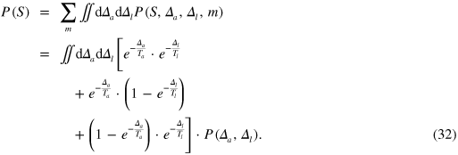
If both  and
and  are independently drawn from equation (21), i.e. if

the fraction of successful trades in the economy would be

A more realistic scenario would be that prices are connected through an exchange rate e as introduced in the third section:

In that case, the fraction of successful trades is

Both cases are depicted in figure 8(b) together with the corresponding simulation results which confirm the analytic solution. In the next section we will see that the introduction of a liquidity market leads to a significantly increased number of successful trades.

Figure 8. (a) Fraction of successful trades in a closed single currency random economy and in a time-homogeneous, symmetric system, both with exponentially distributed transfer prices. The black lines are calculated according to (31) and (36). As one would expect, higher price levels lead to less successful trades since agents simply do not possess enough means of payment to carry out the trades. Due to the additional payment mode, a system of money and antimoney leads to a higher number of successful trades. With the liquidity market switched on, the fraction of successful trades increases even further as agents can now easily obtain means of payment. (b) The fraction of successful trades in a symmetric, time-homogeneous system without a liquidity market for two different price distributions  . The points represent simulation data and the black lines are calculated according to (34) and (36). Of course, in all cases the fraction of failing trades is
  . The simulation was performed with 10 000 agents and
  .
.
Download figure:
Standard image High-resolution image8. The liquidity market
So far we did not make use of the liquidity providing mechanism possible in a time-homogeneous, symmetric system and impossible in a single currency system. Now we switch on the liquidity market such that agents who possess liquidity according to equation (16) will provide it to agents whose trades would otherwise fail because neither the asset holdings of the buyer nor the liability holdings of the seller are sufficient to execute the transfer.
The specific implementation is such that we keep a list of potential liquidity providers and their liquidity. If a trade can neither be executed via money nor antimoney, the buyer will randomly ask agents on that list until the trade can either be realized or there are no more liquidity providers left. In the latter case the trade ultimately fails. We start with the most simple assumption that the price  of liquidity is exogenously given in the simulation. Before we turn to the results of the simulation, let us first calculate the probability of finding an agent who could provide liquidity if the liquidity market is switched off:

As can be seen from figure 9, this describes the simulation results very well. If we now allow liquidity trading, the amount of 'free' liquidity decreases sharply as it is all used up in trades.

Figure 9. The amount of free liquidity in a time-homogeneous, symmetric random economy with and without a liquidity market. Both (a) and (b) show the same data with different scalings for the y-axis. The simulation was performed using 10 000 agents  and
and  . With increasing
  , insufficient liability holdings become the limiting factor for an agent's liquidity according to equation (16). A liquidity market leads to a rapid redistribution of excess liquidity. Note that for
  , prices
  would probably not be encountered in a real economy as this would constitute a loss of monetary wealth for the liquidity provider. The smaller
  , the longer it takes to reach low free liquidity levels. This effect can still be seen for the data point that corresponds to
  . The black lines were calculated according to equation (37).
Download figure:
Standard image High-resolution imageSwitching on the liquidity market also changes the money and wealth distribution. When comparing figures 5(c), (d) with figures 5(a), (b), one can see that the resulting distributions with a liquidity market can still be described by exponential functions except for two 'outliers' in the upper left corner. The outliers represent the liquidity providers who are left with little asset and liability holdings and the buyers of initially failing trades who had to turn to the liquidity market. They end up with smaller asset but larger liability holdings. For the remaining agents we see that the effective temperatures of the fitted exponential distributions (see equation (22)) have changed compared to figures 5(a), (b). Note that this does not mean that  has changed.
Figure 10(a) shows the effective temperatures of assets and liabilities for various prices of liquidity  . In figure 10(b) we have plotted three asset distributions to illustrate the effect. For the liability distributions one would find the reverse effect, i.e. the slopes get shallower with increasing
  . As can be seen from figure 5(d), the wealth distribution is broadened if liquidity trading is enabled. However, for larger values of
  , the wealth distribution becomes increasingly asymmetric, seen in the divergence of the effective temperatures
  and
and  (see figure 10). This makes sense, since buyers of liquidity have to accept more liabilities than assets for
  . A similar asymmetry was found in figure 5(b) for an exchange rate
  . Naturally, the price of liquidity
  also reflects the price levels and thus
  and the exchange rate e are expected to be tightly connected and probably inversely proportional. However, such expectations have to be tested in real economies.

Figure 10. (a) Effective temperatures for different liquidity prices.  is the case of no liquidity market. Note that even for high values of
  , the asset and liability distributions will always be broader than in the case of no liquidity trading. Asset and liability temperatures diverge with increasing
  as the wealth distributions in figure 5(d) become increasingly asymmetric. In (b) we have plotted the asset distribution for three different liquidity prices
  for better illustration of the phenomenon. Note that for increasing
  the slope becomes steeper which corresponds to a lower temperature. For the liability distribution one finds the reverse effect (only shown in (a)).
Download figure:
Standard image High-resolution image
As a final observation, we see from figure 8(a) that the fraction of successful trades is increased when a liquidity market is present. This is to be expected as agents who initially lack liquidity can now turn to the liquidity market and obtain means of payment. Due to the spot trade property, i.e. the absence of long-term contracts (see section 4), this mechanism should be able to alleviate the problem of credit crunches and delayed feedback loops from long-term credit contracts in real systems.
9. Discussion
We analyzed a monetary system of money and antimoney that has only recently become possible with the advent of mobile computers and cryptography. One of the motivations are the non-local effects of credit creation. Once a payment is performed by the creation of credit, the on-setting inflation has an effect on all other market participants. Credit holders profit from the monetary inflation while money holders suffer from the inflation. As a result, the decision between two credit partners influences all other market participants without their consent and without a mechanism to counteract.
Therefore, credit creates a moral hazard. Products are bought by credit creation at price levels before the inflationary effect of the credit and can be sold later at higher price levels after the market equilibrated to the inflationary pulse. This phenomenon can be seen in the contemporary credit crisis. While a small number of banks have profited from the created credit bubble, the resulting crisis is endured by market participants world-wide. It is quite likely that the moral hazard leads to an overboarding credit creation and eventually to periodic debt defaults.
As shown, the proposed monetary structure can prevent this. It is borrowed from the physics of energy and momentum conservation [11] and is inspired by the Noether theorem of time homogeneity. Instead of relying on interest rates to judge the future value of past investments at the time of credit creation, a local exchange rate dynamically compares values of the past (debt = antimoney) with values of the future (savings = money). This judgment is performed in real time by all market participants in any monetary transaction, in stark contrast to interest rate determinations which are judged locally by the subjects of credit creation and typically hold for finite time spans.
The differences from the existing monetary system are rather subtle. Money and antimoney units are normalized to the number of subjects in an economic space. This means that both money and antimoney are issued upon entering and collected upon leaving the economic space. Importantly, money and credit are issued in differing units or currencies. Their mutual value is judged by an exchange rate.
A real implementation of a time-homogeneous, symmetric monetary system has only recently become conceivable with the advent of electronic payment systems. Since the agent's liability units (antimoney) constitute an obligation to render goods or services to society, agents will want to get rid of it. It is obvious that such a system will require one way or another to make the individual antimoney holdings transparent. One would have to make sure that no agent exclusively consumes by accumulating antimoney without ever passing it on to other agents, i.e. without contributing to society. Money on the other hand would not need similarly strict monitoring. For the liquidity market to be efficient, money should preferably be as easily transferable as antimoney. Such a differentiation between money and antimoney would already be possible today: money consists of bank liabilities and non-bank assets while antimoney is memorized as bank assets and non-bank liabilities. Both units are never added or subtracted during monetary transactions and are structurally a money currency and a debt currency [7].
The history of debt is laden with ways of how creditors enforce the payback of loans. An overview from anthropology was recently provided [15]. One rather inelegant possible solution, already discussed in figure 6, would be to impose a debt cap, i.e. transfers would only be allowed if the payer's wealth did not drop below a certain threshold  . Another solution would be to assign time-stamps to antimoney which would determine the period within which the antimoney had to be passed along. This could also be achieved by an electronic implementation. Similar to contemporary structures of inheritance after death, money insurance schemes havee to distribute the risk of subjects leaving the economic space. In this case the same money and antimoney units previously issued upon entering have to be collected. Irving Fisher suggested to choose the amount of central bank money proportional to the total number of market participants [40], an approach that we implemented in our simulations.
The question is whether a market mechanism alone could prevent agents from hoarding antimoney. Closely related to this point is the issue of bankruptcy and defaults. It turns out that the legal framework is likely to be similar to today's rules. If an agent had acquired some good by receiving antimoney and went bankrupt afterwards, i.e. he would be unable to pass on the antimoney within the set time window, the seller had to take the antimoney back and would in turn become responsible again for passing it on. This is the equivalent of a write-off today. Thus, the negotiation of antimoney prices would depend on the buyer's economic standing. For large transaction volumes, financial service providers could provide insurance against an agent's default. Similar to contemporary regulations which implement rules for personal default, an insurance against leaving the system with improper and imbalanced money and antimoney holdings could be implemented. We expect that the exchange rate dynamics between money and antimoney allow other modes of handling liabilities which are not yet conceived from our traditional monetary background using credit and interest.
In the analysis of statistical monetary economies, it is typically assumed that the amount of money is fixed. For this case, it was found early on, that the money distribution follows an exponential Boltzmann distribution [3, 9]. However the quantity of money is not fixed in a modern economy and a free running credit economy leads to a self-contradictory inflation dynamics which can only be kept in check with systematic transfers [7]. Thus statistical economies are very good in checking the robustness of economic systems.
If these transfers are derived from a potential, the Boltzmann distribution can be generalized. Similarly, the mechanism on how a random transfers are forbidden to ensure a fixed quantity of money leads to a predictable wealth distribution. If the amount of money is fixed in a random fractional reserve economy, again an exponential distribution is found [8].
With the above results it comes as no surprise that also for the case of a money–antimoney system, since it fixes the amount of money and antimoney, an exponential wealth distribution is found. However, due to the separation of monies, the negative and positive side of the distribution are independent from each other and follows the respective price levels (figure 5). Even if we enforce a fixed debt cap, the exponential wealth distribution only shifts to the left (figure 6). This simple result allowed us to show that also the distribution of agents who could offer 'credit' by transfer of liquidity—by a simultaneous transfer of money and antimoney—is exponentially distributed (figure 7). We can therefore infer the behavior of the liquidity market in a random money–antimoney economy (equation (36)).
The above results give a solid basis for the subsequent analysis of a liquidity market. If agents are allowed to trade money–antimoney packets with a price of liquidity  , liquidity is very effectively cleared from the market as seen in figure 9. The width of the money distribution is specified with effective temperatures. We find that with the increased flexibility of the liquidity market, the wealth distribution becomes broader (see figures 5(c), (d)). The price of liquidity introduces a small asymmetry into the distributions. We see that the possibility of the liquidity market offers creditary flexibility, but still the distributions converge towards an exponential Boltzmann-like distribution in a random economy, indicating the overall stability of such a system.
How would the market change the prices of antimoney with respect to the prices in money units? At this time we can only speculate and possibly the only answer to this question lies in setting up a suitable experimental setting to probe the dynamics of the exchange rate between the two currencies money and antimoney. The hope and expectation is that the dynamics map to the known structure of the dynamics of two competing currencies of two countries. But without further experimental analysis, we can only speculate on whether the exchange rate between money and antimoney together with the liquidity market could establish a stable market equilibrium by itself. Both the historical record [15] and the most recent credit crises have shown at length that a creditary economy is not providing society a stable market equilibrium.
10. Conclusion
We have introduced a new bi-currency system of money and antimoney that allows exploiting the advantages of full reserve banking systems without giving up easy access to liquidity. Since economic experiments to test the approach are difficult to conduct, we first test the approach within an economic scheme of random transfers. Such stochastic analysis is a good stress test to probe the stability of a monetary system. We provide a number of analytical solutions within that framework. We find that due to the symmetry of the system it is possible for agents to provide liquidity to other market participants without the need for overseeing and enforcing long-term credit contracts on a personal level. This novel mechanism allows one to host a time-symmetric monetary system without inhibiting credit dynamics which would be the case in time-homogeneous systems with only one kind of money.
Acknowledgments
The authors would like to thank Axel Schenzle and Ulrich Schollwöck for discussions and Ludwig Ohl and Robert Fischer for providing feedback on the manuscript at various stages.