


Abstract
Laser–electron beam collisions that aim to generate electron–positron pairs require laser intensities I ≳ 1021 W cm−2, which can be obtained by focusing a 1-PW optical laser to a spot smaller than 10 μm. Spatial synchronization is a challenge because of the Poynting instability that can be a concern both for the interacting electron beam (if laser-generated) and the scattering laser. One strategy to overcome this problem is to use an electron beam coming from an accelerator (e.g., the planned E-320 experiment at FACET-II). Even using a stable accelerator beam, the plane wave approximation is too simplistic to describe the laser–electron scattering. This work extends analytical scaling laws for pair production, previously derived for the case of a plane wave and a short electron beam. We consider a focused laser beam colliding with electron beams of different shapes and sizes. The results take the spatial and temporal synchronization of the interaction into account, can be extended to arbitrary beam shapes, and prescribe the optimization strategies for near-future experiments.
Export citation and abstract BibTeX RIS

Original content from this work may be used under the terms of the Creative Commons Attribution 4.0 licence. Any further distribution of this work must maintain attribution to the author(s) and the title of the work, journal citation and DOI.
1. Introduction
In an intense electromagnetic background, charged particles obtain relativistic velocities and emit energetic photons. A fraction of these photons decays into electron–positron pairs, which can themselves be accelerated by the fields and radiate new photons [1, 2]. The repeated recurrence of photon emission and pair creation leads to the formation of the so-called QED cascades, where the number of particles in a plasma grows exponentially with time.
Pair cascades are believed to affect plasma dynamics in extreme astrophysical environments, e.g., in pulsar magnetospheres and polar caps [3–5]. It was recently proposed that one could re-create a comparable energy density in the laboratory using counter-propagating intense laser pulses [6], which has prompted many scientists to study related configurations using kinetic particle-in-cell simulations [7–27]. As the required laser intensity (I ∼ 1024 W cm−2) is still beyond the extent of the current laser technology, there are many unknowns about the highly nonlinear dynamics associated with plasmas in extreme conditions. Previous proposals [28, 29] have shown that the required laser intensity for copious GeV pair production in near-critical-density plasmas can be reduced to the order of I ∼ 1022 W cm−2.
Before lasers become sufficiently intense to generate dense e+
e− pair plasmas from light, a head-on collision between a pulsed laser and a very energetic electron beam can allow us to generate dilute e+
e− beams by applying the currently available technology [30]. The famous SLAC E-144 experiment has shown the onset of nonlinear Compton scattering and Breit–Wheeler pair production combining a 1018 W cm−2 laser with a  electron beam [31, 32], albeit with a very low positron yield. Experiments are underway, expected to produce more pairs per shot [33]. Research on stochastic effects in radiation reaction is also expected to benefit from the laser–electron scattering experiments [34–38], with new ways to infer the peak laser intensity at the interaction point [39, 40] and probing the transition from the classical to the quantum-dominated laser–electron interaction. Two all-optical experiments have shown the electron slowdown due to radiation reaction [41, 42], but were not able to discriminate between different theoretical descriptions of radiation reaction. We anticipate the near-future facilities (e.g. ELI [43], Apollon [44], CoReLS [45], FACET-II [46, 47], LUXE [48], EXCELS [49], ZEUS [50]) are to probe the electron–positron pair production covering several different regimes of interaction. This manuscript focuses on head-on laser–electron scattering that maximizes the strength of the electric field in the electron rest frame. This is the first experiment planned in most of the aforementioned facilities, and we aim to improve the current predictive capabilities for positron creation.
Due to the inherent non-linearity of the Breit–Wheeler pair production, there is no general roadmap on what would be an optimal strategy to obtain the highest possible positron yield using any given laser system. If the laser is assumed to be a plane wave (adequate when the laser is much wider than the interacting beam), the analytical predictions state that the best strategy would be to use the highest conceivable laser intensity. Therefore it is tempting to conclude that the laser should be focused on the smallest attainable focal spot. Our work shows that this strategy may not always be optimal, as there is a trade-off between the high laser intensity and the size of the interaction volume. With a short focus, the highest intensity region becomes small both transversely and longitudinally, which can reduce the number of seed electrons that interact with the close-to-the-maximum intensity, as well as the duration of this interaction. Using tight focusing also increases the number of particles that are not temporally synchronized with the peak of the laser pulse at the focal plane (these electrons never get to interact with the peak laser intensity, regardless of the transverse position). Finally, the wavefront curvature can also change the effective angle of laser–particle interaction.
Each of the mentioned factors affects the resulting number of positrons; hence a correct optimization strategy would have to take all of them into account at the same time. This can be achieved by resorting to full-scale three-dimensional particle-in-cell simulations, making sure enough statistics is used to represent the interacting electron beam with all its features, as well as high grid resolution in all spatial directions to correctly describe the laser dynamics. This approach requires a lot of computational resources (several million CPU-hours for each parameter set) and can be justified for the support of a specific ongoing experiment where most parameters are not free. However, for future experiments, there are many possible choices. It would thus be practical to devise a simple and cost-effective way for their consideration. This would ensure that the best possible strategies are applied when constructing new laser facilities.
This manuscript aims to simplify the pair production optimization in multi-variable parameter space. The goal is accomplished by extending the analytical scaling laws previously developed for electron interaction with a plane wave to more realistic geometries, taking into account the finite electron beam size and the laser focusing. Our method allows for predicting the number of positrons created in a laser–electron collision with a temporal (longitudinal) or a perpendicular offset. With the model proposed in this paper, predictions can be obtained without simulations. The most demanding calculation required is a numerical integration of an analytical function that can be performed on a single CPU, and the results obtained within minutes. This paper is structured as follows. In section 2, we revisit the pair production in a plane wave. Section 3 covers different methods for calculating the overall positron yield. In section 4, we give predictions for a special case where the electron beam is long and wide compared to the laser beam at the focus. Section 5 discusses a thin electron beam, while section 6 features a short electron beam. Finally, in section 7, we show the optimization of the positron number expected as a function of the available laser and electron beam parameters.
2. Pair production in a plane wave
The simplest description of a laser pulse is a plane wave with a temporal envelope. Such a wave is fully described by the wavelength λ, a pulse duration τ (that defines the extension of the pulse's temporal envelope), and the normalized vector potential a0, which relates to the intensity through ![${a}_{0}=0.855\sqrt{I[1{0}^{18}\enspace \mathrm{W}\enspace {\mathrm{c}\mathrm{m}}^{-2}]}\lambda \enspace (\mu \mathrm{m})$](https://content.cld.iop.org/journals/1367-2630/23/11/115001/revision2/njpac2e83ieqn2.gif) (for linearly polarized lasers). As a relativistic electron interacts with the strong electromagnetic wavepacket, it emits high-energy photons that themselves interact with the laser field and can decay into electron–positron pairs. The process of electron–positron generation is mediated by a real photon through the Breit–Wheeler mechanism [51].
(for linearly polarized lasers). As a relativistic electron interacts with the strong electromagnetic wavepacket, it emits high-energy photons that themselves interact with the laser field and can decay into electron–positron pairs. The process of electron–positron generation is mediated by a real photon through the Breit–Wheeler mechanism [51].
In the plane wave approximation, the total number of new pairs per interacting electron can be estimated if we know the electron energy γ0 me c2 (where γ0 is the initial electron Lorentz factor, me the electron mass and c is the speed of light), and the laser parameters (peak a0, central wavelength λ and pulse duration τ, which is defined as the full width at half maximum of the laser intensity).
The total number of pairs is then given by [52]:

The first term P±(ωc) represents the probability of emitting a photon of frequency ωc; the second is the recoiled χc,rr which accounts for the radiation reaction on the beam electrons and the final term dNγ /dω is the value of the emitted photon distribution at ω = ωc. This approximation underestimates the number of low-energy photons, which does not significantly affect the positron production calculation. According to this model, all positrons are generated from photons with a critical frequency ωc, and there is no feedback by the produced pairs on the photon spectra (in other words, there is only one generation of secondary particles). Furthermore, the model assumes a semi-classical equation of motion of the electrons as they lose energy through the emission of radiation and uses the locally constant field and rigid-beam approximations. This allows for an implicit calculation of the laser phase ϕc at which χ is maximized, which is later used to estimate the emitted photon spectrum and consequently the number of created pairs (figure 1).

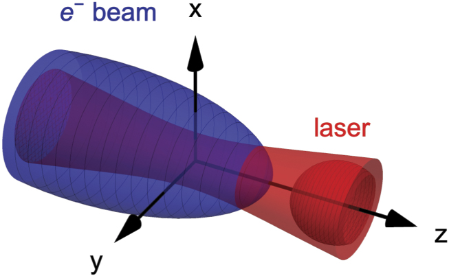
Figure 1. Illustration of an electron beam colliding with a Gaussian laser pulse.
Download figure:
Standard image High-resolution image3. Beyond plane wave
Let us now consider a diffraction-limited laser pulse illustrated in figure 3. The maximum laser intensity an individual particle within the electron beam interacts with depends on two geometrical factors: the transverse offset from the laser axis compared to the laser spotsize and the initial longitudinal position that affects the temporal synchronization of the interaction. In other words, while interacting with a Gaussian laser pulse, electrons far from the focus interact with a lower average (and peak) field, which must be taken into account. The electron encounters the peak of the laser pulse at time t in an (x, y, z) point of configuration space which defines the maximum field felt by this particle. We can therefore assign an effective vector potential a0,eff(t, x, y, z) that corresponds to the maximum laser intensity the particle experiences during the interaction.
We define an equivalent distribution of beam particles according to the maximum intensity they interact with during the scattering. This intensity is identified through the maximum instantaneous vector potential associated with an individual beam particle as a0,eff. In the case of a plane wave interaction, there is no defocusing, and particles always interact with the same intensity, regardless of where or when they overlap with the peak of the laser (a0,eff ≡ a0, and the equivalent distribution, in this case, would be a dirac Delta function). For a more general case, by considering a corrected a0,eff for each particle, we can apply the equations already derived for a plane wave (equation (1)), and then integrate over the distribution function in a0,eff to obtain the total yield of positrons in the laser–electron scattering. The integration can be performed by sampling the distribution function numerically or performing an analytical integration over the configuration space in some special cases where this is possible. In reference [52] the authors calculate the total number of positrons by analytically and numerically integrating the scaling law for the plane wave in full coordinate space x, y, z (for comparison with our predictions cf section 6). The approach in the present manuscript allows to make this procedure shorter and applicable to different beam shapes and sizes. After deriving the distribution of particles dN/da0,eff a one-dimensional integration in a0,eff-space is enough to make predictions on the total number of expected positrons (or some other relevant quantity).
We first obtain a distribution of the interacting particles according to their a0,eff. For every bin in this distribution dN(a0,eff)/da0,eff one can calculate the contribution for pair production using  . This method is cost-effective because it eliminates the need to perform multiple variable integration in the configuration space.
The problem can be addressed using cylindrical coordinate system (ρ, ϕ, z), centered at the laser focus. For a Gaussian laser beam (in the paraxial approximation), the configuration space can be mapped according to the laser intensity isosurfaces shown in figure 2, that do not depend on the coordinate ϕ. For simplicity, let us first assume that the electron beam is a cylinder with a constant density nb. Each particle meets the laser beam at a different point of space, and is assigned a0,eff(ρ, z), where ρ and z are its coordinates at the instant of time when it is synchronised with the peak of the laser. Performing a one-to-one mapping to the new coordinates of a flat-top relativistic beam in counter-propagation with the laser, the beam density in the new coordinates doubles and the length shrinks by two because the laser–electron crossing happens at twice the speed of light. The number of particles dNb(a0,eff) with a0,eff that falls in the interval (a0,eff, a0,eff + da0,eff) can then be estimated to be dNb(a0,eff)/da0,eff = 2nbdV/da0,eff, where dV is the volume between two adjacent isosurfaces associated with a0,eff and a0,eff + da0,eff. Due to the geometry of the problem, this expression can be transformed to the following:

where the surface element  is calculated at the isosurface that is by definition perpendicular to the gradient of the vector potential given by
  .
.

Figure 2. A volume element between two isosurfaces of the effective normalized vector potential a0,eff. The volume element contains all the points where particles experience the peak a0 within the interval (a0,eff, a0,eff + da0,eff).
Download figure:
Standard image High-resolution imageLetting beam plasma density vary in space  allows considering cases of short or long, wide or narrow beams, including non-ideal spatio-temporal synchronization with the laser (as discussed later for cases illustrated in figure 3). It is worth noting that even a point-particle interaction with a Gaussian beam is not equivalent to a plane wave approximation unless the particle is in perfect temporal synchronization with the laser pulse.

Figure 3. Scattering with nontrivial electron beam shapes. (a) A single electron-laser interaction equivalent to electron colliding with a plane wave packet (L ≪ zR, R ≪ W0). (b) Interaction with a long and wide electron beam (L ≳ zR, R ≫ W0). (c) Interaction with a pencil-like thin electron beam (R ≪ W0). (d) Interaction with a short electron beam (L ≪ zR).
Download figure:
Standard image High-resolution imageAn alternative way to obtain the distribution of particles in a0,eff is to numerically sample the electron beam density nb(r, θ, ϕ) in space (the 'sampling' method). The sampled distribution function can be directly binned into a histogram according to the maximum value of a0 each section interacts with. This allows to take into account arbitrary beam shapes, as well as include spatial structure like correlated energy chirp that can be present in LWFA beams. As long as the equation (1) for the number of expected pairs in a plane wave interaction is correct, the 'sampling' method is expected to predict a correct result for a focused Gaussian laser beam interacting with an electron beam of any shape and size. In the rest of the manuscript, we use it as a verification of the explicit distribution functions obtained analytically for several typical cases expected in an experiment. A good agreement between the predictions of the two methods confirms that the analytical distribution functions are correct and that the approximations taken in the electron beam description are valid.
Once the particle distribution in equation (2) is calculated, we can extract field moments  , which can for example be used to calculate the average laser intensity [40].
4. Wide beam
As a first application of the ideas presented in the last section, let us consider the case of the scattering between a focused Gaussian laser pulse and a wide electron beam. The spatio-temporal intensity distribution of a Gaussian laser is characterized by the peak vector potential a0, the laser wavelength λ, and the Rayleigh-range  , where W0 is the transverse spot size. The effective vector potential has the following spatial dependence
  , where z is the distance from the focal plane and ρ is the distance from the laser propagation axis. Our definition of 'a wide beam' is that the beam radius is much larger than the laser focal spot W0. The gradient of a0,eff can be written as
  , where
  . This simplifies the particle distribution in a0,eff according to equation (2):

where the limits of integration in z direction will depend on the beam length and its temporal synchronization with the laser pulse. If the entire isosurface associated with a specific a0,eff is covered with interacting particles,  . Otherwise, a portion of the volume associated with a specific laser intensity may be empty due to the finite beam length and temporal synchronization. The interaction limits imposed by the beam are
  and
and  , where Δ∥ is the longitudinal displacement of the electron beam centre from the focal plane when the laser is at the focus. For every a0,eff, one has to evaluate what the appropriate integration limits are on each side, and there is a transition in the distribution function at values of a0,eff that corresponds to the beam edge on axis. In the case where Δ∥ = 0, the a0,eff above which the iso-volumes are completely full is
  , as shown by the examples in figure 4(a). The distribution function for a centered, wide, flat-top electron beam is given explicitly in table 1. For clarity, the table summarizes the results only for temporally synchronised beams, but the model allows considering more general cases, that are covered in the appendix
We now illustrate the obtained particle distributions according to the effective laser intensity on an example. The SFQED experiment [46] will study pair-production using a 0.61 J laser pulse (a0 = 7.3, λ = 0.8 μm, W0 = 3 μm, τ = 35 fs) and a 13 GeV, 2 nC electron beam. The electron beam follows a non-symmetric Gaussian density distribution transversely with σx
= 24.4 μm, σy
= 29.6 μm, and has a  long flat-top longitudinal profile.

Figure 4. Wide beam, with a flat-top longitudinal envelope. (a) Particle distribution according to the effective laser vector potential a0,eff. Dashed lines are analytical expressions, circles are from sampling and full line corresponds to the limiting case of L → ∞. (b) Positron yield as a function of the longitudinal displacement Δ∥ for one beamlet. The laser parameters are a0 = 7.3, λ = 0.8 μm, τ = 31 fs and W0 = 3 μm. The beam energy is E0 = 13 GeV, transverse width σx = 24.4 μm and σy = 29.6 μm. The beam length is L = 50.9 μm for each beamlet, while the entire beam contains Q = 2 nC and is 250 μm-long.
Download figure:
Standard image High-resolution imageTable 1. Particle distributions according to the effective vector potential for different beam geometries. Here,  is the a0,eff associated with the integration limits imposed by the longitudinal size of the electron beam, Nb represents the total number of particles in the beam, nb is the beam density, R and L are the beam radius and length respectively. The laser spot size is W0,
  is the Rayleigh length, and Δ⊥ is the perpendicular displacement of the beam centre from the laser propagation axis.
| Setup | Particle distribution for temporally centered beams |
|---|---|
| Wide beam |

|
| Thin beam |

|
| Short beam |

|
To save computing time, we performed 3D PIC simulations of this interaction using OSIRIS [53] by dividing the long beam into five equal beamlets each 50.9 μm long. These beamlets have different temporal synchronization (they encounter the laser peak at different distances from the focus). The 3D simulations are performed with a box size of 98 μm × 25 μm × 25 μm, resolved with 3840 × 400 × 400 cells. OSIRIS PIC results (red empty circles in figure 4(b)) are compared with the analytical predictions based on above intensity distribution functions and a numerically sampled beam. The distribution functions for the temporally non-synchronised electron beam with Δ∥ ≠ 0 are shown in the appendix
For the analytical calculations and numerical sampling, we assumed the beam has a uniform density equal to the central density of the electron beam nb = 1016 cm−3. This is justified by σx ≫ W0 and σy ≫ W0, and the highest intensity portion interacts nearly exclusively with the maximum density of the beam. The analytical calculation is therefore coherent with the simulation results, as confirmed by the comparison in figure 4(b).
5. Thin beam
Let us now consider the case of the scattering between a focused Gaussian laser and a long L ≫ zR but thin R ≪ W0 electron beam, where the effective laser intensity can be lower due to a longitudinal offset Δ∥. Here, the problem becomes one-dimensional as the number of particles in the volume associated with a specific value of intensity is given by dNb = 2nbdV = 4nb
S⊥dz = 4(Nb/L)dz, provided that the beam is long enough to interact with the two portions of the same laser intensity before and after the focus (which is always the case if the beam is temporally centered—otherwise if the interaction happens only on one side, the total number of particles should be divided by two). The effective laser intensity depends only on z through  and the distribution can simply be calculated as

Just as in the previous section, the explicit distribution function in a0,eff for a centered beam is given in table 1 (figure 5).

Figure 5. Thin beam. (a) Particle distribution according to the effective vector potential for Δ∥ = 0. (b) Positron yield as a function of temporal synchronization. The beam energy is E0 = 13 GeV, charge is Qb = 1 pC and length L = 200 μm. The laser parameters are a0 = 48.4, λ = 0.8 μm, τ = 35 fs, W0 = 3 μm and Δ∥ represents the longitudinal displacement of the beam centre when the laser is at the focus.
Download figure:
Standard image High-resolution image6. Short beam
Let us now consider a short L ≪ zR beam with a Gaussian density profile  where the peak density is given by n0 = Nb/(πR2
L), x = ρ cos ϕ and y = ρ sin ϕ. We assume a longitudinally synchronized beam (Δ∥ = 0), with an allowed transverse displacement Δ⊥ between the beam centre and the laser propagation axis. The electrons therefore interact with the laser peak at z = 0 and the field structure reduces to
where the peak density is given by n0 = Nb/(πR2
L), x = ρ cos ϕ and y = ρ sin ϕ. We assume a longitudinally synchronized beam (Δ∥ = 0), with an allowed transverse displacement Δ⊥ between the beam centre and the laser propagation axis. The electrons therefore interact with the laser peak at z = 0 and the field structure reduces to  . As the manifolds of constant a0,eff are now concentric rings, the volume element associated with a specific value of a0,eff is given by dV = Lρdρ dϕ/2, the surface element of an isosurface is dS = Lρdϕ/2, and the field gradient is given by
  , with
  . We can now apply the equation (2) to obtain the particle distribution function dNb(a0,eff)/da0,eff = ∫Lnb
ρdϕ/||∇a0,eff||. This gives
. We can now apply the equation (2) to obtain the particle distribution function dNb(a0,eff)/da0,eff = ∫Lnb
ρdϕ/||∇a0,eff||. This gives

where  and the integration result can be expressed through the modified Bessel function of the first kind
  . The obtained particle distribution function is given in table 1 and can be numerically integrated applying
  to every bin of the histogram to obtain the total positron yield from the laser–electron beam interaction. The calculations can be extended to a temporally non-synchronized interaction by replacing a0 and W0 with
  and
and  .
.
In reference [52], the authors consider a spherically-symmetric Gaussian beam profile with a radius R = 6 μm, the laser spotsize W0 = 2 μm and the Rayleigh range zR = 15.7 μm. As the Rayleigh range is much higher than the beam length (zR ≫ R), one can consider the beam short, just like in our calculations. They have obtained an approximate expression for the expected value of the number of positrons, which correctly predicts the order of magnitude, but has a factor of two difference compared with the simulation results in reference [52]. We have applied our distribution functions to calculate the expected number of positrons in this case, and we have obtained the correct result that is consistent with the simulation data of reference [52]. Detailed comparisons are shown in figure 6.

Figure 6. Short beam. (a) Particle distribution according to the effective vector potential for a transversely aligned beam (Δ⊥ = 0). (b) Positron yield as a function of transverse beam displacement from the laser propagation axis Δ⊥. The electron beam energy is E0 = 2 GeV, charge is Qb = 100 pC and Gaussian radius R = 6 μm in all spatial directions. The laser parameters are a0 = 48.4, λ = 0.8 μm, τ = 30 fs and W0 = 2 μm.
Download figure:
Standard image High-resolution image7. Optimal focusing strategy to obtain maximum positron yield
This section covers the optimal focusing strategy for a wide range of laser parameters (in particular as a function of total energy content and pulse duration), as well as different electron beam energies. We assume that the electron beam is 200 μm long (flat-top longitudinal envelope) and has a Gaussian transverse shape. The electron beam is spatio-temporally synchronized with the laser (i.e., the center of the beam interacts with the laser peak at the focal plane, and they share the propagation axis). The transverse beam profile is Gaussian with σx
= 24.4 μm and σy
= 29.6 μm. The chosen on-axis beam density nb = 1016 cm−3 corresponds to the total beam charge of Qb = 2 nC. The results can be scaled to other values for the central beam density by introducing a factor nb/1016 cm−3. A specific laser system has a fixed total energy content, which for a Gaussian transverse profile is approximately given by  . The laser intensity (proportional to
  ) is therefore reversely proportional to the square of the spot size W0. As the number of pairs produced per interacting electron
  is a monotonously rising function of the effective a0, and the number of seed electrons that would experience the high intensity is proportional to the size of the interaction volume
  , to obtain the highest possible number of positrons, one should strike the right balance between a high value of a0 and a large W0. In other words, there is a trade-off between using a short focal length to obtain the highest conceivable laser intensity and having a wider interaction volume where more seed electrons participate in the interaction.
What follows is a calculation of the optimal focal spot and the corresponding pair yield for lasers with energy below 1 kJ and relativistic particle beams with energies lower or equal to 20 GeV. These values include what will soon be available in several experimental facilities (e.g. SLAC [46], HiBEF [54] or ELI [43]).
For each combination of the electron beam energy and the laser total energy content, we apply the analytical expression (see table 1) to calculate the effective a0 distribution of the interacting particles. Then, we integrate the results numerically to find the optimal spotsize and maximum positron yield for this set of parameters (as illustrated in figure 7).

Figure 7. (a) Positron yield as a function of the laser spot size keeping the total energy contained within the laser pulse constant at ɛ = 1 kJ. (b) Optimal spot size for different total laser pulse energies. Beam parameters are E0 = 10 GeV, L = 200 μm, σx = 24.4 μm, σy = 29.6 μm, nb = 1016 cm−3, and we consider τ = 150 fs with λ = 0.8 μm.
Download figure:
Standard image High-resolution imageFigure 8 summarizes the optimization results covering  different parameter combinations, keeping the laser duration constant at 35 fs. For 10 GeV electrons and a 1 kJ laser, a maximum number of pairs is 109, which is obtained using W0 > 8 μm. The FACET-II 13 GeV electron beam at SLAC could generate 4 × 10⁸ pairs/shot if paired with a 300 J laser-focused to W0 = 5.7 μm. The LUXE 17.5 GeV beam with the same laser parameters could produce 7 × 10⁸ pairs per shot, using a slightly larger W0 = 6.8 μm.

Figure 8. Optization study for lasers pulses of fixed duration (τ = 35 fs). (a) Optimal laser spotsize for a head-on scattering as a function of total pulse energy and the electron energy. (b) Positron yield achieved using the optimal spotsize. The laser wavelength is λ = 0.8 μm; the electron beam is L = 200 μm long (flat-top longitudinal profile).
Download figure:
Standard image High-resolution imageSimilarly, figure 9 shows how to obtain optimal results as a function of the laser energy and the laser pulse duration, keeping the initial electron beam energy constant at 13 GeV. This allows estimating the positron yield at ELI Beamlines, where L4 laser specifications are at 1.5 kJ with 150 fs duration. If we assume a third of the laser energy is used to accelerate electrons, 1 kJ is available for the scattering, which can produce 2.4 × 10⁸ (nb/1016 cm−3) pairs per shot using W0 = 6.2 μm.

Figure 9. Optimization study for fixed electron beam parameters (here, electron energy is 13 GeV, corresponding to an accelerator beam available for example at SLAC). (a) Optimal laser spotsize for a head-on scattering as a function of pulse energy and duration. (b) Positron yield achieved using the optimal spotsize. Other laser and electron parameters are the same as in figure 8.
Download figure:
Standard image High-resolution imageThe results presented in this section best correspond to the case of a wide electron beam, which corresponds to a beam from a conventional accelerator. For LWFA beams, the 'thin' beam may be a more adequate description for the laser–electron interaction in some cases (e.g., if the scattering is performed within the LWFA bubble where the electron beam transverse size is  ). We can perform a similar optimization using the thin beam effective intensity distribution functions. If the LWFA beam propagates a few cm before the collision, due to the momentum divergence, the beam size increases, and even an LWFA beam is then well described by the wide beam distribution function.
As an illustrative example, in figure 10 we show the variation in the number of positrons for different values of a0, for synchronized and an offset of 10 μm. In this case, the offset is much smaller than the Rayleigh range, which implies a small variation in the final positron yield.

Figure 10. Effect of longitudinal jitter of laser on the positron yield. Beam parameters are E0 = 3 GeV, L = 10 μm and laser parameters τ = 30.92 fs, λ = 0.8 μm, W0 = 3 μm. The gray area indicates the region for intermediate values of jitter.
Download figure:
Standard image High-resolution imageThe highlighted cases were chosen to reflect the parameters we expect to be available in near-future laser facilities. As time delay and misalignment can be considered, in cases where there are uncertainties about specific experimental parameters, our models can be used as direct support for statistical analysis on pair production. We could incorporate fluctuations in intensity, temporal and spatial synchronization, as well as the fluctuations in electron beam energy distribution, and predict their impact on the final results.
8. Conclusions
The methods outlined in this work allow to make predictions regarding the pair production in laser–electron scattering, taking into account the 3D focusing geometry, spatio-temporal synchronization, and the realistic beam shape and size. This opens a possibility for fast parameter optimization, using analytical calculations directly or combining them with simple numerical integration. The approach is faster than using full-scale Monte Carlo or PIC-QED calculations, and the results can be obtained on a single CPU. Apart from saving computing resources, the ideas from the present study can be applied for real-time optimization and data analysis in experiments.
Besides optimizing the positron yield considered in this manuscript, the equivalent intensity distributions are going to be useful to calculate the asymptotic energy spread [34–37, 55] and divergence of the interacting electron beams [39, 56–58], which are also imprinted on the emitted photon beams in the hard x-ray and gamma-ray range. The analytical description can be generalized to the tight-focusing regime beyond the paraxial approximation (W0 < 2.5λ) considering interaction at an angle for the regions with curved wavefronts. This requires introducing corrections on the effective τ and λ, and considering that the tilted interaction angle directly affects the quantum parameter χ. This will be explored in future publications.
In summary, the findings of this manuscript are expected to be important for near-future laser–electron scattering experiments, as the calculations are fast and can provide real-time feedback during the course of an experiment.
Acknowledgments
The authors thank B Martinez for proofreading the manuscript, as well as L O Silva and T Grismayer for fruitful discussions. This work was supported by the European Research Council (ERC-2015-AdG Grant No. 695088) and Portuguese Science Foundation (FCT) Grant No. CEECIND/01906/2018. We acknowledge PRACE for awarding access to MareNostrum based in the Barcelona Supercomputing Centre.
Data availability statement
The data that support the findings of this study are available upon reasonable request from the authors.
Appendix A.: Distribution in a0,eff for electron beams with imperfect temporal synchronization
In this section, we derive the distribution of particles for an arbitrary temporal synchronization. Similarly, as for the synchronized beams, we map the individual beam particles according to the spatial positions where they encounter the peak of the laser pulse. The temporal synchronization is then quantified through a longitudinal offset of the electron beam center from the focal plane given by Δ∥. Without the loss of generality, we assume that Δ∥ > 0.
To obtain a distribution function in a0,eff for Δ∥ > 0, one needs to evaluate the integral on the RHS of equation (2) between z− and z+, where |z−| < |z+| are the longitudinal coordinates of the edges of the electron beam, given by z± = Δ∥ ± L/4. This integration can be performed formally, but we present a more intuitive calculation relying on geometry. For Δ∥ < L/4, a part of the beam is temporally synchronized with the laser, and some of the particles have their interaction point at the focal plane. This is illustrated in figure 11(a). The beam can be divided into two parts: the blue part on the left-hand side of the focal plane and the yellow part on the right-hand side of the focal plane. The total distribution in a0,eff can then be written as a sum of the distributions coming from the blue and the yellow sections of the beam. Each of these beams contributes with exactly a half of the distribution function associated with a symmetrical (temporally synchronized) beam twice its size. This means we can re-use the distribution functions from table 1, modifying the beam lengths to Lb/4 = |z−| = Δ∥ − L/4 and Lg/4 = |z+| = Δ∥ + L/4. For a large temporal offset Δ∥ > L/4, none of the beam particles interact with the laser in the focus. This is illustrated in figure 11(b). Analogously as in (a), this case can be represented by the symmetric beams distribution functions defined through z±, but this time we subtract the contribution of the blue beam from the contribution of the yellow beam.

Figure 11. (a) A partially synchronized electron beam. (b) Electron beam with a large temporal offset. The beam represented in grey can be expressed as a linear combination of the beams represented in blue and yellow.
Download figure:
Standard image High-resolution image
This reasoning applies both to thin and wide beam geometries. In the case of a short beam, the maximum interaction value for a0,eff will be determined by the distance from the focus through  , and the effective spotsize becomes
  . The modified distribution functions in a0,eff including the temporal offset were collected in table 2 for easy reference.
Table 2. Particle distributions for arbitrary temporal synchronization. The ± sign corresponds to situations where Δ∥ < L/4 or Δ∥ > L/4 respectively, z± = Δ∥ ± L/4. θ(x) is the Heaviside theta function,  and
and  .
.
| Setup | Particle distribution for temporally unsynchronized beams |
|---|---|
| Wide beam |

|

| |

| |
| Thin beam |

|
| Short beam |

|