


Abstract
We develop a theoretical approach to obtain a new differential equation together with a new boundary condition for the density profile of two-dimensional clusters and apply it to the complex plasma case. In addition, we use the local-density approximation for the interaction energy and consider finite size effects. In this case, our differential equation and the previously used reduce to the same. By using the new boundary condition, a scale invariance appears and the obtained scale function can be used in many systems beyond complex plasmas. The obtained equations are confronted with molecular dynamics simulations. We find that the dependence of the system's size and the density profile with the number of particles, N, agrees very well with the results obtained from simulations. The theory has a surprisingly good accuracy for small systems (8 < N < 500). Moreover, we find by simulations that, for a given external potential, the final configuration from an experiment or simulation can provide us, at most, with two possible values for each interaction parameter, the charge and the screening length.
Export citation and abstract BibTeX RIS

Content from this work may be used under the terms of the Creative Commons Attribution 3.0 licence. Any further distribution of this work must maintain attribution to the author(s) and the title of the work, journal citation and DOI.
1. Introduction
In complex (dusty) plasma, monodisperse microspheres of dust can be made to float in a circular monolayer. Electrostatic and gravitational forces are used to confine them vertically. With radial confinement and low temperature, the particles form finite crystalline clusters [1, 2]. The radial potential well is approximately parabolic and is responsible for the circular shape of the cluster. The interaction between dust particles in the plasma is typically subject to shielding by electrons and ions and is therefore frequently described by the Yukawa (or Debye–Hückel) interaction [3, 4].
It is hoped that, given the external potential's parameter, the spatial particle distribution obtained from an experiment or simulation can give values for the interparticle potential parameters by using a suitable theoretical model [5]. In isotropically confined three-dimensional (3D) systems [6, 7], much research has been made toward this direction. The behaviors of the density distribution for many particles [8, 9] and of the shells' structures for few particles (the so-called Yukawa/Coulomb balls) [10] follow well known phenomenological and ab initio equations. These theories give a good accuracy in almost the entire range of the parameters. In two-dimensional (2D) large systems with moderate and strong screening, the continuum density profile was obtained with a satisfactory accuracy [5, 11, 12]. However, the density profile or the system's radius for relatively small number of particles (8–500) and for weak screening (or strong confinement) were not well predicted theoretically.
There are other methods for determination of interaction parameters in Yukawa systems (see e.g. [13]) but macroscopic properties, such as density and radius, can also be investigated in other 2D systems, and the same procedure can be used in many of them. For instance, similar studies were made in systems with pure Coulomb [14], dipolar [15] and superconductor vortex–vortex [16] interactions.
In this paper, we derive good approximations for the density and the radius of 2D complex plasma clusters. The local-density approximation (LDA) with finite size effects (FSE), which were not considered previously in 2D, was used for the interaction energy. By considering deformations in the triangular lattice, which is the predominant symmetry in the system, a new differential equation for the spatial dependence of density is obtained. The general form of this differential equation is different from the ones obtained from others approaches used in the literature [5, 11, 12]. The procedure to obtain this equation helps us to find a new boundary condition which, with the necessary careful considerations, is essential to the accuracy of the final equation. We compare the theory with results of molecular dynamics (MD) simulations and find that it has a surprisingly good accuracy for a great range of the number of particles N, even when the density cannot be considered continuum (8 < N < 500). Moreover, from simulations we found that this system has two regimes where the system's size and density profile are the same but the interaction parameters are different.
Formally, the paper is structured as follows. In the next section the model system and details concerning the MD simulations are given. In section 3, our theoretical approach is developed and, in section 4, their results are compared with those obtained from simulations. Finally, section 5 contains a summary of the main results.
2. Model
With a Yukawa type pair potential  and an external potential Vext(r) = V0r2/2, the Hamiltonian of the system is given by

where N is the number of particles, q is the dust charge, κ is the screening parameter, V0 is the confining potential parameter and α = κ3q2/V0. The rescaled particles' radial positions κri at the ground state are determined uniquely by α and N.
To search for equilibrium configurations of this system, we use a simulated annealing scheme. This is summarized as follows: first, for a given set of parameters, particles are placed at random positions and the solvent is set at a high initial temperature. Then, the solvent temperature is slowly decreased down to T = 0 at a constant rate. The time evolution of the system at a temperature T is modeled by overdamped Langevin equations of motion. These are integrated via Euler finite difference steps following the algorithm

where  is the total force applied to the particle, Δt is the time step and the components of the 2D vector g are independent random variables with standard normal distribution which accounts for the Langevin kicks.
3. Theoretical development
3.1. Interaction energy and the local density approximation
In a continuum approximation for the particle density ρ(r), the total potential over a particle located at r is given by

where Rm is the system's radius. When the range of the potential, 1/κ, is small compared to the system size (i.e. when κRm ≫ 1), a small region around r gives the main contribution to the integral of equation (4). In this case, the effective region of integration is approximately a circle with radius of the order of 1/κ and centered at the position vector r. For such a circular symmetry in the region of integration, we can expand ρ(r') around r (i.e.  ) and one can see that the second term vanishes in the integral of ρ(r') e−κ|r−r'|/|r − r'|. Therefore, the use of just the first term, i.e. of the local density ρ(r), may give a good approximation for ϕ(r). This is called the LDA.
On the other hand, when Rm is equal to a few units of 1/κ or less, FSE must be considered. These effects were taken into account only in the 3D case by Henning et al [9] and we will use a similar FSE consideration in 2D. Even with a constant density, the integral of equation (4) cannot be given in terms of elementary functions. In this case, we consider a position independent FSE by simply integrating over the region |r' − r| ⩽ Rm, i.e. a disc of radius Rm centered at r, which gives

As the system has locally a predominant triangular lattice symmetry, the density is related to the nearest particles' distance x by  . In the limit of strong screening, i.e. a big value of κ and therefore a short range of the pair potential, each particle effectively interacts only with its nearest-neighbors. In this case, the total potential ϕ(r) is approximately equal to 6 (the number of nearest-neighbors of the triangular lattice) times Vpair(x(r)).
Now we make the consideration that each particle in the cluster always interacts with only six effective particles at a distance x (see figure 1(a)) through an effective potential given by Veff(x) = ϕ(x)/6, even when the interaction has a long-range character. In fact, each effective particle is in a nearest-neighbor position but represents the interaction with all the particles in one sixth of the system as is shown in figure 1(a). In the short-range case, the effective potential becomes the pair potential and the effective particles become the nearest-neighbor particles. We considered that the total potential over a particle can be given explicitly in terms of x, i.e. ϕ(r) = ϕ(ρ(r)) = ϕ(x(r)), which is always true for the LDA without a position dependent FSE.
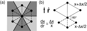
Figure 1. (a) Effective particles and their respective sixth part of the plane. (b) Relative positions of the effective particles in the presence of an external force  .
.
Download figure:
Standard image High-resolution imageEquation (5) is a continuum approximation and therefore it is accurate only when the interaction range 1/κ is much bigger than the particles' spacing x (κx ≪ 1). In fact, for Yukawa systems, this approximation fails when κx ≫ 1, or even κx ∼ 1 [18], and one should consider correlation (discretization) effects. In this case, each particle interacts, effectively, only with few particles in its neighborhood. As those particles have a triangular lattice-like arrangement, we approximate their interaction energy by that given by a perfect triangular lattice. A good approximation for this energy was obtained in [18] by summing up a set of well-defined rings. To include the FSE, we must perform the sum up to the ring of radius ≈Rm, which yields

Notice that in the regime of κx ≪ 1 (or ρ/κ2 ≫ 1) equation (5) is recovered. In the rest of this article, we will use equation (5) and concentrate on 10−4 ⩽ α ⩽ 101. Nevertheless, the already good results obtained for average and great values of α (∝κ3) [11, 12] can still be further improved by using equation (6).
3.2. Differential equation for the density
In order to compensate the external force,  , one must consider a deformation of the original hexagon formed by the effective particles. To do so, we choose the dislocation shown in figure 1(b). In this case, the distance between the central particle and the three effective particles in the positive (negative) direction of
  was increased (decreased) by Δx/2. The angle between two neighbor particles remains π/3 and the total potential remains the same up to the first order in Δx.
The magnitude of the force due to an effective particle is  . Therefore, from figure 1(b) and from the equilibrium of forces, we have

which, for small Δx, becomes

For a smooth dependence of x with r we associate Δx/x to the derivative of x with respect to r. This is based on the fact that the variation of the nearest-neighbor distance from the bottom rhombus to the top one, i.e. the difference between their sides, in figure 1(b), is Δx and the radial distance between their centers is x. By substituting Δx = x(dx/dr) in equation (8), we obtain the following differential equation:

This last equation written in terms of the density becomes

where Vext(r) represents a general external potential.
The obtained differential equation has a general form different from other well-known approaches. In a variational approach [11], the minimization of the total potential energy functional

under the constraint  , gives

Whilst in a hydrostatic approach [12], the Euler equation

where P = −∂(ϕ/2)/∂(1/ρ) = (ρ2/2)∂ϕ/∂ρ is the pressure, gives

In spite of the differences between equations (10), (12) and (14), by using an approximation for ϕ of the form ϕ(r) = Bρ(r), where B is a constant, they provide the same result for the density, i.e. ρ(r) = ρ0 − Vext(r)/B where ρ0 is a constant of integration. The differences between these equations appear when ϕ has other dependences with ρ and r. These differences will be investigated in future work. Now we use the result ρ(r) = ρ0 − Vext(r)/B together with the approximation of equation (5) and the external potential Vext(r) = V0r2/2 to obtain the following equation for the density:

The values of ρ(0)/κ2 and κRm are obtained from the boundary and normalization conditions. As remarked in section 2, they must depend only on the parameters α and N.
3.3. Boundary and normalization conditions
A continuum approximation for the density must satisfy the normalization condition  , which in our case is written as

This equation can be used to eliminate one unknown term of equation (15), while the second one can be eliminated from a boundary condition.
The most simple boundary condition is to say that ρ(Rm) = 0. However it does not indeed happen, although becomes a good approximation in the large N limit where, as observed in experiments and simulations, limN→∞ρ(Rm)/ρ(0) = 0 ∀α. The use of this condition and equation (16) in (15) gives

where

Except by the factor (1 − e−κRm) descendant from FSE, this result was obtained by Totsuji et al [11] by using a variational approach. There, the result ρ(Rm) = 0 comes out from the minimization of the total energy obtained from the LDA without FSE and correlation effects. When the latter effects were considered [11], a non-zero density at the edge came out naturally, satisfying limN→∞ρ(Rm)/ρ(0) = 0.
Notice that, from the effective particles approach of figure 1(b), a straightforward boundary condition appears. When the central particle of figure 1(b) is at the boundary of the cluster, the three effective particles at the top do not exist. Therefore, the equilibrium of forces considered in equation (7) is now written as (1 + 2 cos(π/3))F(xm) = V0Rm, where xm is the nearest-neighbor distance at the boundary, or equivalently

Despite the consideration of just three effective particles in this case, the effective potential continues to be given by ϕ(x)/6. This is in fact a correction for our choice of the term (1 − e−κRm) for the FSE. This choice overestimates the potential at the edge by a factor that approximates the number 2 as κRm increases.
By placing the potential ϕ of equation (5) into equation (19) we obtain an expression relating xm and Rm

An important and non-trivial consideration must be made here: for a particle at the edge, just a fraction of its Wigner–Seitz cell is inside the circle of radius Rm (see figure 2). This fraction is approximately one half for Rm/xm > 1. Due to this fact, the density (given by the inverse of Wigner–Seitz cell area) at the edge is related to xm by

This correction in the density should be made always that the superior limit of integration of the normalization condition shown in equation (16) is Rm. In this case, the total area occupied by all Wigner–Seitz cells must be equal to πR2m but it is overestimated if we always have  (see figure 2). This problem has not been considered previously in the literature but it becomes important in small systems. Equation (21) is not exact but gives a good approximation to correct this problem.
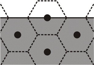
Figure 2. A particle located at the edge of the system has only a half of its hexagonal Wigner–Seitz cell inside the circle of radius Rm.
Download figure:
Standard image High-resolution imageUsing equations (21) and (20), we obtain
The above equation is one of the main theoretical results obtained in this paper. It will be determinant for the good accuracy of the theory at small number of particles. By using equation (22) in equation (15), we can find ρ(0) in terms of Rm. Finally, the density at any point is then given by
where κRm can be found by using equation (16), which gives
3.4. Scale invariance
For a given number of particles, equations (23) and (24) inform that the distances in the system scale with Rm, i.e.

where f(N,r/Rm) is independent on the potentials' parameters. This would imply that the values of κ and α cannot be obtained separately from the final configuration of an experiment, but only from a relation between them. Another experiment with a different N must be done in order to get a new relation.
A density profile obeying equation (25) can be obtained when the potential ϕ is, up to a constant, approximated by ϕ(r) = Bρ(r). By using this approximation, the method of the previous two subsections (i.e. any of equations (10), (12) and (14) together with  and equation (19)) gives

where c = c(N) is obtained from

and Rm is related to B by

The factor B can be a function of N, Rm and of the potentials' parameters; and may be obtained, for example, by: (a) an integral of the pairwise potential  , as it was done in equation (5), or (b) by a derivative of the Madelung energy (equation (6)), B = ∂ϕ/∂ρ, evaluated at the mean density
  . Indeed, the approximation ϕ = Bρ is very general and can be used in many systems beyond Yukawa [16, 17], and so does equations (26) and (27).
The scale invariance of the theory is broken when position dependent FSE (small κRm) or correlation effects (small ρ/κ2) are taken into account. Using the latter, Totsuji et al [19] were able to obtain approximate values of κ and q2, for a given V0, by considering the α-dependence of R2mρ(0). Their results are applicable with the assumption that α ≫ 1. But, as we will see in section 4, if all values of α are possible a priori, α can be a bi-valued function of R2mρ(0).
4. Results
Equations (24) and (26) for the radius and the density, respectively developed in the latter section, were compared with the results obtained from MD simulations in order to verify the accuracy of our theory.
We defined the system's radius as the radial distance of the outermost particle. Although, in the theory, we have made considerations that demand great values of κRm and ρ/κ2, which implies in the need of great number of particles since  , we still found satisfactory results even for N < 500. Figure 3(a) shows the N-dependence of κRm, obtained from equation (24) (lines) and simulations (symbols) for α = 101, 1, 10−1, 10−2, 10−3 and 10−4. In figure 3(b), we compare equation (24), equation (24) using
  instead of equation (21), equation (18) and the equations obtained in [12] and [11] (with cohesive energy) in the case of α = 10−2.
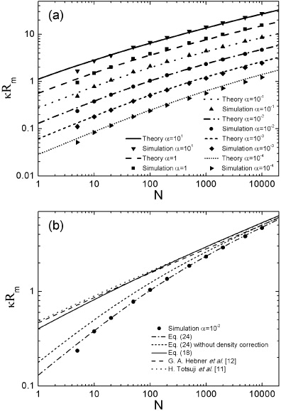
Figure 3. (a) Scaled radius κRm versus number of particles N in logarithm scale obtained from simulations (symbols) and equation (24) (lines) for α = 1, 10−1, 10−2, 10−3 and 10−4. (b) Comparison between our theoretical results and the ones developed in [12] and [11].
Download figure:
Standard image High-resolution imageThe surprisingly good agreement of the theory for small number of particles is evidenced in figure 4 where α = 10−2 and no logarithm scale is used. The dotted and dashed lines represent equations (18) and (24), respectively. One can see that the boundary condition of equation (22) was responsible for a great improvement in the theory.
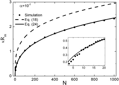
Figure 4. Scaled radius κRm versus number of particles N in normal scale for α = 10−2 obtained by equation (24) (dashed line), equation (18) (dotted line) and by simulations (symbols). The inset shows a zoom for 2 < N < 21.
Download figure:
Standard image High-resolution imageThe inset of figure 4, which is a zoom for 2 < N < 21, shows that, although the radius obtained from simulations has a discontinuous dependence with N, the theory gives a good smooth approximation. A good accuracy starts as N > 8, when the structural transition (1,7)↦(2,7) occurs for all α [20]. For N ⩽ 8, the particles are located at the vertices of a regular polygon centered at the origin with one or none particle at the center. In these cases, the exact values of κRm can be easily obtained theoretically. For α = 10−2, the relative error of equation (24) is less than 5% for any N > 8.
The radial density profile was calculated by dividing the system in annuli and counting the number of particles in each annulus. This number is then divided by the area of the respective annulus and the result is taken as the density at the mean radius of the annulus. For a smooth profile, the width of the annuli cannot be too small. Such smoothness can only be obtained for  .
.
Since the accuracy of the theory for the radius is already known from figure 3, we now investigate the accuracy for the density by showing only how R2mρ depends on r/Rm. By doing this, the scale invariance predicted by the theory in section 3.4 is also investigated. Figure 5 shows R2mρ versus r/Rm for many values of α (the same of figure 3(a)) and for (a) N = 10 000, (b) N = 1000 and (c) N = 100. In the figure the results from our theory are shown, which is given by equation (26) and does not depend on α, and from the one developed in [11] (with cohesive energy) for α = 10−4 and 101 (the curves for other values of α are between the two and so are the ones obtained by the theory of [12]). As it can be seen, our theory gives a good approximation even for values of N between 100 and 1000, which are more easy to be achieved in experiments.

Figure 5. Scaled density R2mρ versus scaled radial distance r/Rm obtained by the theory (line) and by simulations (symbols) for several values of α and (a) N = 10 000, (b) N = 1000 and (c) N = 100.
Download figure:
Standard image High-resolution imageWe can see from figures 5(a) and (b) that the density behavior is approximately parabolic and depends on α. We interpolate this density using a one-parameter fitting function given by

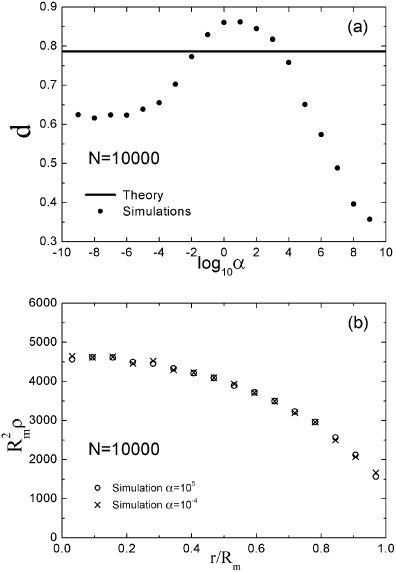
where d = d(α,N) is the fitting parameter. This function is parabolic on r and attends the conditions of equation (16) and of continuity of its gradient for |r| < Rm. Figure 6(a) shows the values of d for N = 10 000 as a function of α obtained by interpolations of equation (29) with simulation results (symbols) compared with the value predicted by the theory (line). We can see that the fitting results have a well-behaved dependence on α. However, it is not injective, i.e. it does not have a one-to-one correspondence. For instance, the scaled densities of α = 10−4 and 105, for N = 10 000, are shown in figure 6(b) and one can see that they are almost the same. This implies in a limitation of any theory for the density: there can be two possible values for each of the system's parameters (κ, q and V0) which can result in the same values of Rm and ρ(r) coming from an experiment or simulation. Also, just a theory which accounts non-local, finite size and correlational effects can predict these two regimes at the same time, giving the two possible values of the parameters.
Figure 6. (a) Coefficient d versus α obtained by interpolations (symbols) and by theory (horizontal line). (b) Scaled density R2mρ versus r/Rm obtained from simulations for α = 10−4 and 105.
Download figure:
Standard image High-resolution image
5. Conclusions
The density profile and the system's size of 2D complex plasma clusters confined by a parabolic potential are obtained analytically. For the calculation of the interaction energy, we used the LDA with a position independent FSE. A differential equation for the density was obtained by a new method. By using the proposed interaction energy, this differential equation gives the same result of the variational [11] and pressure [12] approaches, however our method gives light to an important new boundary condition.
The density resulted from our approximation scales with the radius, implying that the values of κ and α cannot be calculated separately from the final configuration of a single experiment. In fact, the real density does not have this scale invariance but it is showed that there are systems with different α but identical normalized density profiles.
The boundary condition and the FSE were determinant to provide surprisingly good results in systems with relatively small number of particles (8 < N < 500). For instance, for α = 10−2, the relative error of the theoretical maximum radius is less than 5% for any N > 8.
Acknowledgments
The authors thank L Q Costa Campos for his help in the improvement of our simulations. This work was supported by FACEPE (Fundação de Amparo à Ciência e Tecnologia do Estado de Pernambuco), grant numbers APQ-1352-1.05/10, APQ-1800-1.05/12 and BIC-0493-1.05/12.