
Abstract
Dielectric Elastomer Actuators (DEAs) are elastic parallel plate capacitors consisting of polymers as dielectric layer and compliant electrodes'. In dynamic applications with high frequencies DEAs heat up. In this work the heating is studied by experimental investigations as well as by modeling of the visco-elastic behavior of the polymer and the specific electric resistance of the electrode and of the polymer. The experimental investigations have also been performed, in order to obtain parameters for the material model. A partially coupled thermo-electro-mechanical material model is presented and used for the numerical simulations. The experimental and numerical results for the time-dependent thermal behavior show an excellent qualitative correlation. This confirms the quality of the developed multi-field model.
Export citation and abstract BibTeX RIS

Original content from this work may be used under the terms of the Creative Commons Attribution 4.0 license. Any further distribution of this work must maintain attribution to the author(s) and the title of the work, journal citation and DOI.
1. Introduction and state of the art
Dielectric elastomer actuators (DEAs) are smart structures, which are built as compliant capacitors with an elastic dielectric layer sandwiched between two compliant electrodes', made from graphite [1], metal [2] or carbon nanotubes [3, 4]. By applying an electric potential, the electrostatic attraction between the electrodes' leads to a deformation of the elastic dielectric structure. The working principle of DEAs is shown in figure 1.
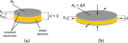
Figure 1. Structure and working principle of a dielectric elastomer actuator. (a) initial state, (b) deformed state after applying an electrical voltage to the electrodes'.
Download figure:
Standard image High-resolution imageThe dielectric elastomer film contracts in thickness direction and, as it is incompressible, expands in lateral direction. Detailed information on the capabilities and properties of DEAs are given in Carpi et al [5]. The operation principle is already well known. An early description of experiments with rubber as dielectric material can be found in the publication of Röntgen [6] from 1880. Due to progress in material sciences and fabrication methods, investigations of dielectric elasomers came back to interest, leading to an early modeling approach of Pelrine et al [7]. In 2000, Kornbluh et al [8] referred to viscoelastic behavior but still used Pelrine's linear elastic modeling approach. Some early experimental investigations, including viscoelastic behavior, were performed by Benslimane and Gravesen [9]. The need for considering the viscous contributions into the mechanical models for the simulation of DEAs were recognized and implemented for example in the model by Ask et al [10]. This model is based on the multiplicative split of the deformation gradient into elastic and viscous components and an additively splitted energy function, including contributions for elastic and viscous response. A non-linear numerical model for visco-electroelasticity was presented by Büschel et al [11] by regarding hyperelasticity. Mößinger et al [12] used an extended lumped parameter model including damping, for numerical investigations of the transient electromechanical behavior of DEAs. A model in analogy to the Kelvin-Voigt model, with additive decomposition of the Piola-Kirchhoff stress tensor, was shown by Madsen et al [13]. In a model of Schlögl and Leyendecker [14] the damping parameter dependent viscous amount is represented by an additive split of the Piola-Kirchhoff stress tensor. The model used in this paper equals the one used from Wissler and Mazza in [15]. Here, a Prony series is used to implement time dependent behavior. A different approach was used in the thermodynamic model from Lucking Bigué et al [16], by employing experimental loss factors, providing an amount of power 'lost' or rather transformed into heat.
Previous experimental investigations have shown, that excitations with fast alternating voltages, lead to a significant heating of a DEA [17]. Localized heating due to spikes in [electric] current where observed from Dudata et al [18]. Christensen et al [19] presented an electro-thermal model to analyze the thermal breakdown, depending on the number of layers in a stack actuator. In this model only resistive heating is studied. By also considering the mechanical deformation, a thermo-electro-mechanical model has been developed and presented in [20].
The aim of the present investigation is to study the primary causes for power loss and enhance the simulation model by experimental data, to explain the observed heating of a given DE-structure undergoing a cyclic load.
2. Experimental investigations
In order to be able to select an adequate material model for the numerical simulation of DEAs, its behavior has to be investigated experimentally. The behavior is based on the structure and the working principle of the DEA and can be divided into a mechanical and an electrical part. With the experimental investigations described in this section the mechanical and electrical material behavior of a sample DEA will be determined.
The structure of the sample DEA is shown in figure 2 and its geometrical parameters are listed in table 1. It consists of 49 stacked elastic dielectric layers with an active area of 40 mm diameter. For the electrical connections of the 50 electrodes', the active area is surrounded by a 5 mm passive region. The thickness of the elastic dielectric layers hd
is 45 µm, the thickness of the electrode layers he
is 5 µm. Hence, the thickness of the whole DEA is about 2.5 mm. The dielectric layers are made of the silicone ELASTOSIL P7670 from Wacker Chemie AG. The electrodes' consist of graphite particles MF2 from NGS Naturgraphit GmbH. For connecting the electrode layers, copper wires are put into the passive electrode area.

Figure 2. Top view and cross section of the sample multilayer DEA.
Download figure:
Standard image High-resolution imageTable 1. Parameters of a DEA module.
| Description | Value |
|---|---|
| Number of active dielectric layers n | 49 |
Thickness of dielectric layer 
| 45 µm |
Thickness of graphite electrode 
| 5 µm |
Diameter of active area 
| 40 mm |
Total diameter 
| 50 mm |
2.1. Mechanical behavior of dielectric elastomers
The mechanical behavior of the DEA primarily results from the mechanical properties of the elastomer. The silicone used as elastic dielectric shows an elastic and viscoelastic behavior. It behaves isotropic and is incompressible with a Poisson's ratio of ν ≈ 0.5.
The deformation behavior of an elastomer can be represented by a stress-strain curve. To obtain this curve, a uniaxial compression test with the measurement setup shown in figure 3 is carried out. The compression tests were performed to reach deformations which resemble the ones during operation. For testing, samples of ELASTOSIL P7670 with 2.5 mm thickness and 5.8 mm diameter are prepared. The test samples are compressed between the lubricated adapters with a velocity of 0.01 mm s−1 and the resulting force is measured. The engineering stress is calculated by dividing the measured force by the size of the initial area on which the force is acting. The engineering strain is calculated by dividing the length change by the initial length of the sample.

Figure 3. (a) Measurement setup for uniaxial compression tests, (b) adapter and test sample before testing and (c) during testing.
Download figure:
Standard image High-resolution imageAlthough the mechanical behavior of the DEA primarily results from the mechanical properties of the elastomer, the influence of the graphite powder electrodes' should be known. Because it is not possible to do the compression tests with loose graphite powder, test samples with the same dimensions as the silicone test samples are cut out of the active area of a DEA and again the uniaxial compression test is carried out. Figure 4 shows the obtained stress-strains curves of the pure ELASTOSIL P7670 and the actuator test samples.

Figure 4. Stress-strain diagram of the uniaxial compression test, the duration of one cycle is 290 s.
Download figure:
Standard image High-resolution imageIt can be seen that the graphite electrodes' in the DEA sample lead to a steeper stress-strain curve compared to the pure silicone sample. In addition, both curves show a hysteresis which is due to the viscoelastic properties of the silicone.
The time-dependent viscoelastic behavior is described by creep and relaxation processes. Creep means that if the elastomer is subjected to a constant mechanical stress step it responds with an initial strain step followed by an exponential increase of the strain over time. Relaxation is the asymptotic decrease in stress over time after an initial stress step due to an applied strain step (see Zhao et al [21]).
For determining the viscoelastic behavior of the ELASTOSIL P7670 and the DEA a creep test and a relaxation test were performed. For the creep test, a test sample was subjected to a constant force which results in an initial compression strain of about 20 %. During the relaxation test a constant compression strain of 25 % was applied to the test sample. Displacement respectively force were measured for 20 minutes. The determined creep and relaxation curves are shown in figures 5 and 6. The forces needed for a compression of about 20 % differ for the pure silicone sample and the actuator sample. In case of the actuator, the force needed is higher because as seen in the stress-strain curves the actuator behaves stiffer than the pure silicone due to the electrodes'. For this reason, the resulting stress in the actuator is higher for a constant compression of 25 % as in the silicone sample. However, the silicone and the actuator samples show similar time-dependent creep and relaxation behavior.

Figure 5. Compression creep test of ELASTOSIL P7670 and actuator, (a) stress vs. time, (b) strain vs. time.
Download figure:
Standard image High-resolution image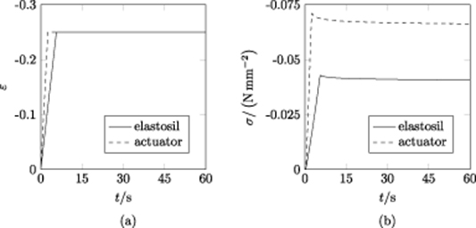
Figure 6. Compression relaxation test of ELASTOSIL P7670 and actuator, (a) strain vs. time, (b) stress vs. time.
Download figure:
Standard image High-resolution image2.2. Electrical behavior of dielectric elastomers
The DEA setup can be transformed into an electrical equivalent circuit, which is shown in figure 7. It consists of the capacitance  , the parallel resistance of the dielectric polymers layers
  which causes the leakage current and the series resistance
  which includes the electrode resistances and the contact resistances of the electrical connections [22].

Figure 7. DEA equivalent circuit with parallel resistance of the polymer..
Download figure:
Standard image High-resolution imageThe value of the capacitance  can be calculated by
It is defined by the material properties of the elastic dielectric (vacuum permittivity  0, relative permittivity
  ) and the actuator design (active region A, thickness of the dielectric layer
  ).
).
A direct measurement of the relative permittivity  of the dielectric layer is impossible. Therefore, a sample structure is fabricated. Copper electrodes' with a defined size are sputtered on a silicone membrane with 50 µm thickness. With an LCR meter the capacitance of the sample structure is measured and the relative permittivity is calculated after rearranging equation (1):
The value of the calculated relative permittivity  of ELASTOSIL
 P7670 is 3.
In general, the value of the parallel resistance  of unmodified silicone material is of the order of gigaohms up to teraohms. For ELASTOSIL
 P7670
P7670  is about 40 GΩ [23]. With
  the specific resistance results to around 1 TΩ cm.
As already mentioned, the electrodes' consist of graphite powder particles. For this type of electrode a constant specific resistance, as it is valid for homogeneous materials, does not exist. But it is possible to measure the sheet resistance  which is defined as
with  as specific resistance and
  as electrode thickness. For the sheet resistance measurement a sheet resistance meter is used. The measured value for the graphite powder electrodes' is 10 kΩ. By rearranging equation (3), the value of
  is calculated. With the given electrode thickness of 5 µm the specific electrode resistance
  results to 5 Ω cm.
In this work the contact resistances are neglected. But previous measurements have shown that the used type of electrical connection results in contact resistances at the transition from compliant electrodes' to the stiff copper wires between 10 kΩ and 80 kΩ [24].
2.3. Electro-Mechanical coupling
The application of an electric voltage to the DEA leads to an electrostatic attraction between the electrodes'. The effective electrostatic pressure  can be calculated by [7]:
The electrostatic pressure depends on the relative permittivity  of the elastomer, the applied voltage U and the thickness
  of the dielectric elastomer layers. The voltage applied to the DEA is restricted by the dielectric breakdown field strength of the elastomer. Taking into account the thickness
  of the elastic layers and the breakdown field strength of the material a maximum voltage can be calculated. However, it is important to take into account the varying thickness of the layers.
After the application of the electric voltage the DEA deforms until the electrostatic pressure is balanced by the elastic pressure of the elastomer. The resulting deformation of the DEA depends on the mechanical material properties of the elastomer. The stiffer the material, the smaller the deformation.
Figure 8 shows the measured actuator strain depending on the applied electric voltage and field strength for the sample DEA introduced before. In figure 8(b), the straight line represents the electric field, i.e. the voltage over the actual thickness, and the dashed line the voltage over the initial thickness. This means that for a given strain the actual electric field is larger than the prescribed nominal one. Due to the breakdown strength  of ELASTOSIL
 P7670 with at least 30 V µm−1 the maximum applied voltage U during testing is 1200 V. This leads to an electric field strength E of around 26 V µm−1 taking into account the thickness change of the elastomer layers. At the maximum applied voltage the deformation of the DEA is about 9 %. For the thickness measurement two laser displacement sensors (Keyence LK-G32) are used. During actuation, the deformation of the DEA is measured from both sides [25].
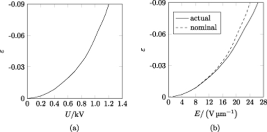
Figure 8. Characteristic deformation curve of actuator, (a) voltage versus strain and (b) electric field versus strain, here nominal means the electric field is calculated with E0 = U/ .
.
Download figure:
Standard image High-resolution image2.4. Thermo-Electro-Mechanical coupling
Dielectric elastomer actuators heat up during operation. This heating up due to dynamic excitation is a thermo-electro-mechanical process. On the one hand this is due to the non-ideal conductivity of the electrodes' and the contact resistances and on the other hand this is due to the visco-elasticity of the elastomer. During operation of the DEA, charging and discharging current is flowing through the electrodes' and a leakage current is flowing through the polymer. Because of the resistances, the electric current leads to a heating along the electrodes' and at the electrical connection of the DEA. In addition, heating in the elastomer material occurs due to the deformation of the material and the appearing internal friction of the molecules and due to joule heating. The increase of temperature in the DEA depends strongly on the dynamic excitation. In general, DEAs are used at frequencies f of the electric voltage from DC to around 1 kHz.
For measuring the heating of the sample actuator, a voltage U of 1 kV at frequencies f of 10 Hz, 100 Hz and 1 kHz is applied for 30 minutes to the electrodes'. During this time the temperature of the whole DEA is measured with a thermal imaging camera (FLIR SC655). Figure 9 shows the thermal images of the tested DEA after 30 seconds and 30 minutes operation with 1 kHz and 1 kV. A symmetric temperature distribution was obtained after 30 seconds, as expected. The temperature distribution after 30 minutes was not symmetric. This behavior may be caused by an uneven degradation of the left and the right electrical connections of the DEA. The temperatures at the two points marked in figure 9 are analyzed and the results are shown in figure 10. The diagrams show the influence of the frequency to the heating of the DEA. With increasing frequency the temperature in the actuator increases as well. In addition it can be seen, that during operation the DEA heats up slowly in the middle of the active area and much faster next to the electrical connections. For higher frequencies the area next to the connections reaches a temperature of almost 125 °C and the heating process seems not to be finished. The region in the middle of the actuator reaches temperatures between 33 °C and 45 °C.

Figure 9. Thermal images of the sample DEA subjected to a dynamic excitation of 1 kV and 1 kHz, (a) after 30 seconds and (b) after 30 minutes. The sample actuator was filmed from the side.
Download figure:
Standard image High-resolution image
Figure 10. Heating of the test DEA due to the frequency of the applied voltage, at point No. 1 and Point No. 2. see figure 9, experimental data.
Download figure:
Standard image High-resolution image3. Multi-Field model
In the present section, the physical models of the involved mechanical, electrical and thermal domains are presented. Both, the coupling of the mechanical and electrical domain, as well as the mechanism of the resulting heating of the cyclic actuated structure are given.
3.1. Mechanical field
To evaluate the mechanical behavior of the DE structure, a model is needed, which is capable of describing visco-hyperelastic behavior. The aim of this section is, to (i) present the mechanical field equations and (ii) introduce the applied mechanical material model.
In the following equations the index notation is used, as well as the Einstein summation convention for the coordinate indices k, l, m = 1, 2, 3. The deformation gradient tensor  is given by:
Here,  represents the current position vector and
  the referential position vector. The deformation gradient can be decomposed polarly into a rotational and a stretch component

where  is the rotation tensor,
  is the (material) right stretch tensor and
  is the (spatial) left stretch tensor. The eigenvalues of
  and
and  are called the principal stretches λp
. In this work, the material is assumed to be incompressible, which leads to
are called the principal stretches λp
. In this work, the material is assumed to be incompressible, which leads to

With the mass density ϱ, the Cauchy stress tensor  and the volume force density vector
  the balance of momentum reads

 is the second order time derivative of the current position vector. The symmetry of the stress tensor

follows from the balance of angular momentum. Regarding the assumption of incompressibility, the hyperelastic material behavior can be described according to Ogden [26], for which the strain energy density W is defined as
with the material constants µi and αi . By including time-dependence of the material parameters, represented in terms of Prony series, a viscoelastic material behavior can be modeled [27].
The parameters for the Prony series are  , βj
and τj
. The exponential decay in stiffness has been proved appropriate to model the mechanical behavior of silicone subjected to cyclic loads [28]. Thus, the principal values of the Cauchy stress σp
can be calculated as
, βj
and τj
. The exponential decay in stiffness has been proved appropriate to model the mechanical behavior of silicone subjected to cyclic loads [28]. Thus, the principal values of the Cauchy stress σp
can be calculated as
where  is an arbitrary hydrostatic pressure introduced due to the incompressibility constraint equation (7). Please note, that there is no summation over indices given in brackets.
3.1.1. Dissipation in the mechanical field.
To investigate the energy which is converted into the thermal energy during the actuation, the mechanical energy 'loss' has to be considered [29]. Therefore, we define the mechanical power density  as
as

For further investigation we additively decompose the mechanical power into an elastic  and a viscous part

In the case of cyclic loading, the sum of the elastic mechanical power vanishes over each cycle due to the equilibrium of the mechanical energy of the loading and unloading phase. The mean value of the viscous mechanical power density  can be calculated from the potential energy density u lost in each cycle and the frequency of the mechanical loading function

As shown in figure 11, the 'lost' potential mechanical energy density in each cycle, which is transferred into thermal energy, is equal to the area of the hysteresis in the stress-strain-diagram.

Figure 11. Schematic representation of the mechanical hysteresis of the viscoelastic behavior; the 'lost' energy density per cycle u is shown within the hysteresis loop.
Download figure:
Standard image High-resolution image3.2. Electrical field
The electrical field formulation has to be considered in the two components of a DEA, (i) the polymer, where the electric potential leads to a polarization of the dielectric material and (ii) the electrode, where the electric charge is mobile. The balance laws of the electrical field are derived from Maxwell's equations. If we neglect magnetic effects, the Maxwell-Faraday equation is defined as

for which  represents the third order Levi-Civita-tensor and
  is the electric field vector. Gauss's law

provides a relation between the electric displacement field  and the density of the free electrical charge
  . From Ampère's circuital law

we obtain the third balance equation, where  denotes the free current density. The continuity of charge provides the formal relation of charge and current
Here, the superscript  and
and  stand for the free and bound parts of charge and its current. For the electric field in the dielectric material we assume a linear, isotropic material behavior

Here, 0 stands for the free space permittivity and  for the relative permittivity. While charging and discharging, the constitutive equation for the current is given by
where ρ represents the respective specific resistance.
3.2.1. Dissipation in the electrical field.
For the dissipation in the electrical field two effects have to be considered, the dielectric loss and the resistive loss.
The dielectric loss occurs, due to the fact of dielectric relaxation. The loss tangent (or the dissipation factor) is considered to be small for silicone rubbers within the investigated frequency range (with the maximum of  ) [30]. Thus the dielectric power loss is assumed to have a minor influence on the heating of the structure and will be neglected in this work.
The specific resistance of the electrode leads to a loss while charging and discharging the electrode layers. Due to the scales of frequency and the strength of the electric field investigated, for this work only the resistive loss is considered. The power density of an electric current within an electric field  is given by

Considering the constitutive equation (21) the density of the resistive power loss  can be calculated by

if the current on the electrodes' is known. For the dissipation, resulting from the leakage current flowing through the polymer [31], we can determine the power loss density depending on the electric field in the dielectric material by
3.3. Electro-Mechanical coupling
For the electro-mechanical coupling, we use the additive decomposition of the total stress tensor  into a mechanical part and the Maxwell stress tensor [32]

The mechanical stress tensor  is equal to the previously defined Cauchy stress. The Maxwell stress tensor
  is defined as
where  . Considering compliant electrodes, this formulation is consistent with the previously equivalent electrostatic pressure in equation (4).
3.4. Thermal field
Since DEAs are subjected to a heating and therefore a temperature change, the thermal field has to be incorporated. The thermal field is described by the heat equation
Here χ denotes the specific heat capacity, κ the thermal conductivity, T the temperature,  the convective heat flux vector and
  the total volumetric heat source. At the top and lateral surfaces of the DEA a convective cooling is assumed as boundary condition, which is dependent on the difference between surface (
 ) and ambient (
 ) temperature and the heat transfer coefficient α.

The heat transfer coefficient itself depends on the difference between surface and ambient temperature as well [33].


Please note the different dimensions of α and β. The used values for the variables are given in table 3. The surface normal vector  is defined by the boundary of the thermal field. The former defined power losses in equations (15), (23) and (24) are supposed to completely transfer into heat

With these assumptions the thermal field is fully defined.
4. Numerical simulation
In this section, it is described, how the system of equations (presented in section 3) is solved numerically. Therefore, the numerical tools Matlab and Ansys are used. Due to the different time scales of the processes regarding the respective fields, the computation was performed in several substeps. The thermal field, for example, is evaluated within a duration of 30 min, employing time steps of seconds. Much smaller time steps are necessary to compute the mechanical behavior with a cyclic excitation of up to 1000 Hz. A fully coupled analysis would have made it necessary to perform the simulation with time increments defined by the fastest process, leading to a vast amount of required computational power, to simulate the examined actuator.
For the numerical simulation in Ansys two test cases are investigated, for which the geometrical parameters are given in table 2.
Table 2. Geometric dimensions and characteristics of the test-DEA.
| Stack | Unit Cell Test Case 1 | Unit Cell Test Case 2 |
|---|---|---|
| number of active dielectric layers n = 49 |
 heat transfer constant lateral surface heat transfer constant lateral surface


|


|
The first one (test case 1) uses a round electrode similar to that used by the DEA in the creep and relaxation test, described in section 2.1. Test case 2 is defined as the sample DEA, shown in figure 2, with alternating mirror symmetrical electrode design. Figure 12 shows the workflow of the numerical simulation, performed in this work, in order to calculate the heating of the actuator, resulting from the electro-mechanical excitations. First, the material model parameters are obtained from a curve fitting procedure, on the basis of the experimental data given in section 2. Second, the mechanical material model is evaluated by numerical simulations using the finite elements software Ansys. For that, the geometry of test case 1 is employed. As third step, a coupled transient electro-mechanical simulation is performed for the same test case. For this operation, the input is given by an application of a sinusoidal voltage on the electrodes'. As result we obtain the displacements as well as the stress  and strain
  response versus time. From that data, the power loss due to the viscous loss
  is calculated. The data of the resulting electric field within the polymer is used to determine the power loss due to leakage current
  . Additionally, via the data of the electrodes' charge density
  , the free current density
  at the electrode and derived from that the electrodes' resistive loss density
  are computed, within the forth step of the solution procedure. Therefore, test case 2 is used for the simulation of the electrical charging and discharging of the electrode. For a thermal analysis (step five), in which (i) a constant input of thermal energy and (ii) a temperature-dependent convection is prescribed. The temperature in the probe increases with time resulting in a steady-state solution. The heat input is given with the power losses
  and
and  calculated in the previous steps. Convective cooling is applied on the upper and lateral surface. This simulation will provide the resulting temperature distribution versus time. To not unnecessarily inflate the calculations, the following assumptions are made:

Figure 12. Illustration of the solution procedure.
Download figure:
Standard image High-resolution image4.1. Homogeneity of mechanical field
It is sufficient to only distinguish between the active and the passive domain, since the mechanical field is assumed to be homogeneous within the excited layers. The intersection of these domains with an inhomogeneous mechanical behavior is small in comparison to the rest, so that by neglecting this intermediate domain the occurring inaccuracy will be insignificant.
4.2. Neglecting of edge effects of electric field
5. Parameter identification, results and validation
The experimental investigations performed in section 2 were used to obtain the necessary parameters for the material models in section 3, employed for the simulation described in section 4. In the present section, the simulation results are given. In section 5.1 the material parameters are provided. The correlation of experimental and numerical results of the mechanical behavior is given in section 5.2. In section 5.3, the results of the thermal simulations are given and validated with the experimentally gained heating curves for the investigated frequencies.
5.1. Parameter identification
The parameters for the mechanical model are obtained from a curve fitting procedure between the mechanical material model and the experimental data of the relaxation test. The mass density of ELASTOSIL P7670 is taken from the manufacturer data sheet [36]. The mass density of the electrode is assumed to be equal to the one of the polymer. Since we use the experimental data of the actuator, the mechanical model assumes a homogenized structure of the actuator in thickness direction. The electrical material properties were measured as described in section 2.2. The parameters for density, thermal conductivity and specific heat of silicone rubber were taken from results available in literature [37, 38]. Since the structure of the electrode is not exactly known, there exist no really reliable data. Empirical values have been used, resulting from previous numerical investigations. A list of the used material parameters is shown in table 3.
Table 3. Material parameters of the numerical simulation.
| Description | Symbol | Value |
|---|---|---|
| Mechanical material properties | ||
| Ogden-model stiffness | µ1 |
|
| µ2 |
| |
| µ3 |
| |
| Ogden-model exponent | α1 | 1.3 |
| α2 | 5 | |
| α3 | −2 | |
| Prony-model decay factor | β1 | 1.3 × 10⁻¹ |
| β2 | 7.5 × 10⁻² | |
| β3 | 2.3 × 10⁻² | |
| Prony-model decay time | τ1 | 2.2 × 10⁻² s |
| τ2 | 4.0 × 10⁻¹ s | |
| τ3 | 3.2 × 101 s | |
| mass density | ϱ |
|
| Electrodynamical material properties | ||
| relative permittivity of polymer |

| 3 |
| specific resistance of electrode |

|

|
| specific resistance of polymer |

|

|
| Thermodynamical material properties | ||
| thermal conductivity of polymer |

|
|
| thermal conductivity of electrode |

|

|
| specific heat capacity of polymer |

|
|
| specific heat capacity of electrode |

|
|
| heat transfer constant top surface | βT |
|
| heat transfer constant lateral surface | αL |
|
| heat transfer constant lateral surface | βL |
|
5.2. Results of the simulation of the electro-mechanical field
The results of the electro-mechanical simulation are presented in this section. The electrostatic attraction of the electrodes', due to the excitation with a sinusoidal voltage, leads to cyclic stress in thickness direction. The resulting strain becomes stationary after a certain number of cycles, as consequence of the viscous material behavior. The envelopes of the strain are displayed in figure 13, for the frequencies of  . Since the difference of energy loss per cycle within the transient part is small with respect to the duration of the complete process, we only consider the stationary behavior for the subsequent analysis.

Figure 13. (a) Sinusoidal voltage excitation, filled background marks the amplitude of the oscillation and (b) the envelope of the response strain, the stationary state is established in a few seconds.
Download figure:
Standard image High-resolution imageFigure 14 shows a hysteresis plot, resulting from the numerical simulation. Here, the difference of the loading and unloading phase in one cycle at the frequency of 1 kHz is given, for when this difference becomes stationary. The abscissa is given by the curve of the loading phase. The area within the curve is equal to the viscous energy lost per cycle, as described in section 3.1. Whereas the viscous power loss and the power loss due to leakage current are evenly distributed in the active domain, the electrodes' resistive power loss is not. The charging and discharging related current density on the electrode layer is distributed as shown in figure 15, with peaks at the connections of the wires. At these locations the electrodes' current density has a maximum, thereby also the power loss owns its maximum there, compare equation (23). In table 4, the numerically obtained values of the viscous power loss density  , the polymers resistive power loss density
  and the maximum of the electrodes' resistive power loss density
  are given for the investigated frequencies. Comparing the sources of power losses by the proportion of the cumulated amount, one finds out, that the total viscous power loss
  is quite small and does not contribute significantly to the heating of the DEA. For frequencies up to
  , the leakage current in the polymer is the dominant cause for the total power loss. At higher frequencies, the electrodes' resistive power loss becomes the major contributor of the total power loss.

Figure 14. (a) Exemplary hysteresis plot, (b) Difference between the loading phase (lower graph) and unloading phase (upper graph) of the sinusoidal excitation of  and
and  .
.
Download figure:
Standard image High-resolution image
Figure 15. (a) section used for numerical investigation (half model), using symmetry conditions, (b) normalized distribution of the electric current  on the electrode layer.
Download figure:
Standard image High-resolution imageTable 4. Calculated power loss density for examined frequencies.
| Frequency |

|

|

|
|---|---|---|---|

|
|
|

|

|
|
|
|

|
|

|

|
Nevertheless, the local heating of the structure is primarily defined by the local values of the power loss density p. For all investigated frequencies, the hot spots always occurred at the wires, which can be explained (i) by the superposition of all three regarded contributions for power loss and (ii) by the maximum of the electrodes" resistive power loss density  in this area.
5.3. Results of the simulation of the thermal field
In this section the results of the thermal field analysis are given. For this, the input load for the heat generation due to mechanical and electrical power losses were determined in section 5.2. In figure 16 the thermography of the DE test-structure is shown, gained by the numerical simulation with a cyclic excitation of  and
and  . As expected, the highest temperatures occur at the connection wires. As can be seen, the whole structure heats up with increasing time. For locations at point No. 1 (in the middle) and point No. 2 (near the hot spots) the computed temperatures versus time are shown figure 17. One may notice, that the temperatures are higher for higher frequencies.
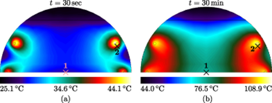
Figure 16. Plot of the numerically computed surface temperature of the sample DEA subjected to a dynamic excitation of  and 1 kHz, (a) after 30 seconds and (b) after 30 minutes. (Please consider the different temperature scales).
Download figure:
Standard image High-resolution image
Figure 17. Heating of the test DEA due to the frequency of the applied voltage, at point No. 1 and point No. 2 (see figure 16), computed results.
Download figure:
Standard image High-resolution image
6. Conclusion and outlook
In the present research, the thermal behavior of a dielectric elastomer test-structure under a cyclic electro-mechanical load was investigated, both experimentally and numerically.
In the experimental part, the thermo-electro-mechanical behavior of dielectric elastomer actuators has been investigated: for a cyclic actuation, the heating of the composite structure consisting of polymer and electrode layers has been studied. It has been shown, that the temperature increases with time and is maximal near the electrical connections. The obtained mechanical and electrical parameters are used for the numerical study.
In the modeling and simulation part, a one-way coupled thermo-electro-mechanical material model is presented. By using a linear electrical model and a visco-hyper-elastic mechanical model, the dissipation of the energy-transformation and thus the heat production was calculated, in order to obtain the input for the simulation of the thermal field. Concluding, this generated heat leads to a temperature increase of the DE test-structure, until a thermal equilibrium is reached. We have shown that the mechanical dissipation leads to a very low global heating in the active domain, whereas the electrical dissipation leads to a much higher heating, which is inhomogeneous in the electrodes'. This inhomogeneous heating reaches a maximum at the wires, as expected.
It has been shown that the experimentally and numerically obtained surface temperatures of the DEA match quite well. The maximal values in the experiment are a little bit higher than in the numerical simulation. This confirms that an application of temperature-dependent material parameters and the integration of thermal degradation phenomena are necessary. Also it is necessary to determine strain-dependent electrical parameters (e.g. resistivity and permittivity) as also mentioned by [39]. These aspects will be investigated in further research.