
Abstract
Non-equilibrium vibrational dissociation CO2 → CO + O at translational–rotational temperatures T ⩽ 1200 K is investigated with semi-empiric and computational models. The governing parameter  has been introduced, where Q is the specific volumetric power coupled into vibrational states and n0 is the initial number density of CO2. It has been shown that the non-equilibrium vibrational process can only be triggered when
  exceeds some critical value determined by the speed of vibrational relaxation. Simple semi-empiric calculations are backed by the state-to-state simulations of the CO2 vibrational kinetics in two-modes approximation performed for conditions of microwave sustained gas discharges. The vibrational kinetics model is benchmarked against the experimental vibrational relaxation times as well as the shock tube data on the rate of the process CO2 + M → CO + O + M for M = Ar and literature data for M = CO2. At T = 300 K the estimated
  W m3 or
  35 W (m−3 Pa−2) (p is the gas pressure).
  is found to always increase with increased T.
Export citation and abstract BibTeX RIS

Original content from this work may be used under the terms of the Creative Commons Attribution 4.0 licence. Any further distribution of this work must maintain attribution to the author(s) and the title of the work, journal citation and DOI.
1. Introduction
Plasma chemical conversion of CO2 into CO is intensively studied now as a potential upstream process for production of synthetic fuels and chemicals (power-2-X) [1–3]. Initially those studies were inspired by, presumably, very high energy efficiency of the CO2 conversion in microwave plasmas reported in the past [4, 5]. The chemical energy efficiency ηchem up to 80% achieved at relatively low translational–rotational temperatures T ≲ 1000 K was ascribed to dissociation from high vibrational states in conditions of strong vibrational non-equilibrium [4–6]. The reported high efficiencies at low T were not reproduced later. In the modern day experiments the highest ηchem of 40%...50% are observed at T > 2000 K and are largely explained by thermal quenching [7–10]. Nevertheless, activating the non-equilibrium conversion mechanism remains an attractive option for increasing the efficiency of plasma processes to make them in this respect competitive with electrolysis.
The non-equilibrium vibrational conversion can be triggered when the kinetic energy of electrons is deposited predominantly into excitation of vibrational states. The electron kinetics calculations had undefined shown [11–13] that this shall be indeed the case for reduced electric fields typical for the microwave plasmas. This condition is necessary, but not sufficient. In order for the dissociation from high vibrational states to be eventually activated the speed of relaxation of vibrational energy with the translational–rotational degrees of freedom must be slower than the speed of the chemical process. Vibrational relaxation in CO2 and its connection with activation of the non-equilibrium CO2 dissociation is the subject of the present paper.
Since the non-equilibrium mechanism of dissociation has not been undoubtedly detected in plasma experiments the theoretical and computational analysis is indispensable for understanding how its activation could be achieved. A simple consideration based on the semi-empiric vibrational relaxation equation known from shock tube and sound absorption experiments [14, 15] suggests that the activation of the non-equilibrium dissociation is controlled by the governing parameter  , where Q is the specific (volumetric) power input into vibrational states, and n0 is the initial number density of molecules. The non-equilibrium process can be triggered when the parameter
  exceeds some critical value. To obtain quantitative estimates and verify the result of the semi-empiric theory this latter is supplemented by a computational study performed with a 0D state-to-state vibrational kinetics model.
There is no generally accepted 'standard' way of modelling the vibrational kinetics of CO2. Unlike for diatomic molecules one cannot describe each single vibrational state with an individual particle balance (master) equation because the number of states is prohibitively large. Therefore, all existing state-to-state CO2 models use one or the other kind of 'coarse graining' [16–19]. An extensive account on the subject can be found in [20]. For the present study the 'two-modes model' [21] is applied where the treatment of vibrational levels is simplified by combining symmetric stretching and bending vibrations into one effective mode. This is an approximate model with restricted quantitative accuracy which main purpose is verification and extension of the semi-empiric approach. The modelling study is divided into three steps, or into consideration of three model systems:
- (a)A test which mimics the conditions behind a shock front. Its purpose is to check that the vibrational kinetics model is properly calibrated to reproduce the empiric relaxation times.
- (b)Thermal dissociation of CO2. The results are compared with shock tube measurements of the rate of the process CO2 + M → CO + O + M for M = Ar, and with literature data for M = CO2. This benchmark indicates that at least for T > 2000 K the model is able to reproduce the correct orders of magnitude of the dissociation rate.
- (c)The model calibrated, verified and partly validated in the two previous steps is applied to study the onset of the low T non-equilibrium vibrational dissociation in conditions relevant for microwave plasmas.
On the step (c) in a series of numerical experiments it is shown that the rate of the primary dissociation process CO2 → CO + O rapidly increases starting from zero when  is increased above some critical value. The critical value of
  as well as that of the critical vibrational temperature are found to be not sensitive with respect to model uncertainties. The
  calculated by the semi-empiric formula agrees well with the results of numerical simulations.
The rest of the paper is organized as follows. The next section summarizes the analytic and semi-empiric treatment of vibrational relaxation in CO2, introduces the governing parameter  and the criterion of activating the non-equilibrium dissociation. A brief overview of the two-modes model, underlying assumptions and constrains is given in section 3. Sections 4–6 describe the numerical experiments with the model systems listed above, including the comparison of the two-modes simulations with experimental data and analytic formulas. Section 7 puts the theoretical results presented in the paper into the context of the current CO2 plasma conversion research. Last section gives a summary of the main findings and a brief outlook on the prospective of future work.
2. Analytic and semi-empiric treatment of vibrational relaxation in CO2
2.1. Summary on vibrational relaxation equations
The basic information about vibrational relaxation in molecular gases is obtained in shock tube and acoustic experiments [14, 15, 22]. Here for compactness the consideration is structured around relaxation in shock waves. Same relaxation processes take place in sound waves and the relaxation rates deduced from both types of experiments agree [15, 22]. Behind shock wave fronts a very rapid increase of translational temperature is followed by its fast equilibration with rotational temperature. The characteristic time of translational–rotational relaxation is  sec at atmospheric pressure (see [14], sections 48 and 49). The thermal excitation of vibrational states is much slower: the typical characteristic times at 1 bar are 10−6...10−5 s. At the same time, unless the temperatures are not very high, the change of the gas composition due to chemical reactions takes place on a significantly longer time scale.
It is well known that for a gas of diatomic molecules with unchanging number density the relaxation of vibrational energy after instant increase of translational–rotational temperature T can be described by a simple differential equation, see e.g. [14], chapter 19:

Here Evibr is the average specific vibrational energy per molecule,  is the average vibrational energy per molecule at Boltzmann equilibrium with temperature T, τ is the relaxation time which depends only on T and on the number density of collision partners M (see below) nM
:
is the average vibrational energy per molecule at Boltzmann equilibrium with temperature T, τ is the relaxation time which depends only on T and on the number density of collision partners M (see below) nM
:

where R10 is the rate coefficient of transition from the first vibrationally excited state to vibrational ground state, ℏω is the energy of one vibrational quantum. In this simplest case of one-component gas nM equals to the number density n of the molecules themselves. Here and below, unless specified explicitly, the temperatures are always expressed in energy units.
Equations (1) and (2) are derived on the following assumptions: (i) the molecules are linear (harmonic) oscillators; (ii) the probabilities of vibrational–translational (VT) transitions can be calculated by a first order perturbation theory: e.g. SSH (Schwartz–Slawski–Herzfeld) or Landau–Teller theory; (iii) the number of vibrational states is infinite. For CO2 which has three modes of oscillations (1) and (2) have to be modified. Two more assumptions are added: (iv) exchange of vibrational energy with translational–rotational modes proceeds only via transitions between the bending mode oscillations:

(v) exchange of energy between bending modes  and stretching modes v1, v3 is very fast. Here Herzberg notation of vibrational states is used, see [23]. Rigorous derivation under assumptions above can be found in appendix


here ℏω2 is the fundamental energy of bending oscillations v2.  is calculated by applying the known formula for harmonic oscillators, see e.g. [24], equation (49.3) there. Factor 2 takes into account that the mode v2 of CO2 is double degenerate. R10 is the rate coefficient of the process:

In [25] it had been shown that when a system of linear oscillators initially has Boltzmann distribution with temperature equal to the translational–rotational temperature T, and T is instantly increased, then vibrational relaxation towards final equilibrium state proceeds via a sequence of Boltzmann distributions with vibrational temperature Tvibr ⩽ T. The result of [25] is not directly applicable to CO2, but numerical experiments presented in section 4 below confirm its validity in that case as well. For the Boltzmann vibrational distribution equation (4) is transformed into equation for Tvibr which can be easily integrated:

Here  is the (dimensionless) heat capacity due to vibrational modes which is calculated by applying the formulas for linear oscillators, see e.g. [24], equation (49.4):
ℏωi are the fundamental energies of the three modes of CO2 oscillations.
The assumption of Boltzmann distribution of vibrational levels allows to derive one more equation where the rate of vibrational relaxation appears explicitly—by transforming (4) into equation for Evibr-2:

One can see that the rate of relaxation (subsequently, the instant relaxation time) is not independent of Tvibr, but this dependency is weak. The factor  only changes from 1 at low Tvibr where c2 ≫ c1, c3 (because ℏω2 < ℏω1, ℏω3) to
  at high Tvibr where c1, c2, c3 → 1.
Equation (9) suggests the following approximation. One can assume that the total vibrational energy Evibr decays with exactly same rate as Evibr-2, and then apply equation (1) with τ defined as:

with  being some average temperature, e.g.
  where T0 is the initial Boltzmann temperature before the vibrational relaxation starts. Of note is that a relation similar to (10) appears also in [22], equation (24) there.
To estimate the accuracy of this approximation a comparison is made with numerical solution of equation (7) with constant T. Both solutions are expressed in terms of the dimensionless time:

That is, the explicit dependence on nM and R10 is eliminated. The temperature Tvibr obtained by solving (7) is translated into Evibr by the linear oscillator formula:

The fundamental energies of the CO2 oscillations [26]: ℏω1 = 0.167 83 eV, ℏω2 = 0.083 427 eV, ℏω3 = 0.297 10 eV. The time evolution  is compared with the exponential function:

where t is replaced by t' and τ is replaced by  , see (10) and (11). The relative difference
  between two solutions is defined as:

where the maximum is taken over the time interval from t' = 0 to t' = 10 ⋅ τ'.
For the test with T0 = 300 K and  the quantity is found to be always ⩽5% for T ⩽ 2500 K. This outcome means that, provided that all the assumptions underlying (7) are fulfilled, the time evolution of Evibr can be approximated with good accuracy by equation (1) with τ defined by (10). This characteristic time, in turn, depends on the rate coefficient of only one process (6). The coefficient R10 then serves as a single parameter which fits the vibrational kinetics model into experimental data.
2.2. Threshold of the non-equilibrium vibrational dissociation
There is a direct link between the rate of vibrational relaxation and the activation of the non-equilibrium vibrational dissociation in a gas discharge. This link can be found by the following simple consideration. In the most general terms the balance of vibrational energy of the CO2 molecules is written as:

where n is the number density of CO2 molecules, Q is the power deposited into their vibrational modes, QVT is the rate of the energy losses into translational–rotational modes, and Qdiss is the rate of vibrational energy losses into chemical transformations. For the dissociation from the upper vibrational states to be significant their population has to be high enough, that is, Tvibr—or Evibr—has to increase up to a certain high value. For this to happen at low translational–rotational temperature T the right-hand side of (15) has to be larger than zero (n ≈ const. before the dissociation starts).
In the near threshold regimes where Qdiss < QVT the last term can be neglected. The term QVT can be written in the form suggested by equation (1):

where  is the empiric energy relaxation rate coefficient.
At constant T the term (16) monotonically increases with increased Evibr so that with Qdiss = 0 the solution of (15) would finally arrive at some nearly stationary value  required for efficient dissociation to start. For this critical
  the equality
  is approximately valid. Since only the very beginning of the conversion process is considered it can be taken that n = nM
= n0, where n0 is the initial CO2 density before the process starts. Then the threshold (critical) value of
is approximately valid. Since only the very beginning of the conversion process is considered it can be taken that n = nM
= n0, where n0 is the initial CO2 density before the process starts. Then the threshold (critical) value of  which corresponds to the critical
  is readily found as:

The criterion (17) has a simple physics meaning. For the vibrationally non-equilibrium process to start the rate of producing the vibrationally excited states has to be at least as fast as the rate with which vibrational energy is transferred into translational–rotational modes.
To apply the equation (17) in practice  and
and  must be known. RVT can be extracted from experimental data, but for
  there is no simple estimate. The main goal of the model system studies which will be presented below in sections 4–6 is to find plausible estimate of
  and to verify the simple formula (17) by comparing it with the results of detailed vibrational kinetics simulations. It will be shown that empiric RVT obtained in shock tube experiments are valid approximately for the conditions of microwave plasmas as well. One will also see that the term in square brackets
 ![$\left[\dots \right]$](https://content.cld.iop.org/journals/0963-0252/31/9/094002/revision2/psstac882fieqn34.gif) in (17) which comes out of the simulation results does not vary a lot from case to case. The magnitude of the corresponding vibrational temperature
in (17) which comes out of the simulation results does not vary a lot from case to case. The magnitude of the corresponding vibrational temperature  —around 3000...4000 K—coincides with the expectations based on the shock tube dissociation data (see section 5).
Prior to that main study the assumptions behind equation (7) will be verified (section 4) by the same state-to-state vibrational kinetics model which is later used for the microwave discharge study in section 6. It will be shown that they hold, and in a certain temperature range the state-to-state model calibrated as prescribed by equation (10) does reproduce the experimental relaxation times τ with good accuracy. The experimental data which are used for both calibrating the state-to-state model and defining  in equation (17) are outlined in the next subsection.
2.3. Experimental data on the rate of vibrational relaxation in CO2
The experimental data on VT-transfer in CO2 had been commonly published in form of relaxation times τ defined in terms of equation (1). The experimental τs could be reduced to functions of translational–rotational temperature T only [15, 22]. The most recent review found on the subject is the publication [27]. When comparing that paper with the older report [28] one finds no references on process (6) with M = CO2 which had not been taken into account in [28]. Therefore, here the rate coefficient of process (6) as a function of T is taken from [28] (process  , M = CO2, in table IIIa there) as the best fit of the all available experimental data. Apparently, this rate coefficient was obtained by applying equation (2) with ℏω = ℏω2 rather than equation (10). The correctness of this assumption is confirmed by translating the rate coefficient back into
  , and comparing the result with selected primary publications on the relaxation time measurements. This comparison is shown in figure 1 where
  'reverse engineered' as described above ('Blauer–Nickerson 1973') is plotted together with results of the shock tube [15, 29] and sound absorption [30, 31] experiments. The agreement is very good.
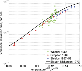
Figure 1. Experimental characteristic time of vibrational relaxation τ, see equation (1), at pressure 1 bar. 'Weaner 1967' is [29], 'Simpson 1969' is [15]; 'Shields 1967-59' is [30, 31] as reproduced in [15]. Solid line is the fit from [28].
Download figure:
Standard image High-resolution imageThe rate coefficient of process (6) applied in the present work is calculated by using equation (10) with τ derived from the rate coefficient  of that process in [28]. That is:

The coefficient  corrected in that way is fitted by the equation:

Here T is in Kelvin and the resulting R10 is in m3 s−1. For T from 250 K to 2000 K (19) approximates (18) with maximum relative deviation 0.5%. The magnitude of the correction factor was already discussed in section 2: the original and corrected rate coefficients are nearly equal at low T, and R10 is twice as large as  at high T (⩾2000 K).
Finally, the coefficient  for equation (17) is calculated from the coefficient
  by applying (2) backwards:

3. The model of CO2 vibrational kinetics in two-modes approximation
There are at least two readily available vibrational kinetics models of CO2 developed primarily for the spacecraft atmospheric entry problems which include full manifold of vibrational levels. The model of Kustova et al [17, 18, 32–34] and the model of Vargas et al [19]. In the model [17, 18, 32–34] the states  with same rotational number l are combined into effective states
  . When all vibrational states up to dissociation limit are included in the model there are in total approximately 8000 master equations to integrate. A 1st order perturbation theory—Schwartz–Slawski–Herzfeld (SSH) model [14]—is applied for calculation of the probabilities of transitions between effective states. The model [19] is a modern development which uses completely different approach. In [19] the master equations are written for the individual modes of oscillations rather than individual or effective vibrational states. Their number is reduced to 250. To calculate the transition probabilities the non-perturbative forced harmonic oscillator (FHO) model [35] is applied. Moreover, in the model [19] the process of CO2 dissociation itself is modelled in detail. Whereas in [17, 18] Treanor–Marrone model is applied to calculate the dissociation rate in [19] the transition from singlet ground state X1Σ to electronically excited triplet state 3
B2 via potential surfaces crossing is modelled explicitly as well as subsequent vibrational kinetics of the state 3
B2. According to shock tube studies the 'forbidden' transition X1Σ → 3
B2 is the dominant channel of CO2 dissociation [36].
. When all vibrational states up to dissociation limit are included in the model there are in total approximately 8000 master equations to integrate. A 1st order perturbation theory—Schwartz–Slawski–Herzfeld (SSH) model [14]—is applied for calculation of the probabilities of transitions between effective states. The model [19] is a modern development which uses completely different approach. In [19] the master equations are written for the individual modes of oscillations rather than individual or effective vibrational states. Their number is reduced to 250. To calculate the transition probabilities the non-perturbative forced harmonic oscillator (FHO) model [35] is applied. Moreover, in the model [19] the process of CO2 dissociation itself is modelled in detail. Whereas in [17, 18] Treanor–Marrone model is applied to calculate the dissociation rate in [19] the transition from singlet ground state X1Σ to electronically excited triplet state 3
B2 via potential surfaces crossing is modelled explicitly as well as subsequent vibrational kinetics of the state 3
B2. According to shock tube studies the 'forbidden' transition X1Σ → 3
B2 is the dominant channel of CO2 dissociation [36].
The model of Vargas et al is physically much more accurate than the models based on the 1st order perturbation theories and is likely to substitute them in future. Nonetheless, those latter have the advantage that they are based on straightforward textbook physics theories and their numerical implementation is relatively simple. Thus, they still suit well for preliminary investigations preceding more advanced computational studies. The model applied in the present work is of such 'preliminary' kind and is based on the 1st order perturbation theories similar to the model of Kustova et al. The main issue of that latter is too large number of equations which have to be integrated making its implementation computationally challenging [34]. The solution of that problem is further coarse graining by grouping the vibrational states. One of such methods is the 'adaptive energy bin' technique proposed in [37, 38] which is applied to couple the full vibrational kinetics including all levels up to dissociation limit with hydrodynamics.
In the present work the study is restricted to 0D simulations and conceptually more simple approach is applied—the so called 'two-modes approximation' [21]. This approximation originates from the well known fact that the  states with the same good quantum number vs = 2v1 + v2 have very close vibrational energies. Thus, it is plausible to assume that the relaxation between those states is fast. In addition, some of them are in Fermi resonance, see [23, 28], which adds to increasing the speed of mutual relaxation. Experimental information about the real speed of energy exchange between symmetric stretching and bending modes v1 and
  is very scarce [27], and in two-modes approximation it is taken as postulate that this relaxation is always faster than all other relevant time-scales of the system. Therefore, all vibrational states
  with same vs can be gathered into combined states
 ![${\mathrm{C}\mathrm{O}}_{2}\left[{v}_{\mathrm{s}},{v}_{\mathrm{a}}\right]\ ({v}_{\mathrm{a}}={v}_{3})$](https://content.cld.iop.org/journals/0963-0252/31/9/094002/revision2/psstac882fieqn50.gif) . Moreother, to derive the formulas for effective probabilities of transitions between combined states it is assumed that the energies and populations of the elementary states within one combined state
. Moreother, to derive the formulas for effective probabilities of transitions between combined states it is assumed that the energies and populations of the elementary states within one combined state ![${\mathrm{C}\mathrm{O}}_{2}\left[{v}_{\mathrm{s}},{v}_{\mathrm{a}}\right]$](https://content.cld.iop.org/journals/0963-0252/31/9/094002/revision2/psstac882fieqn51.gif) are exactly equal. This is an extreme assumption, but it greatly simplifies the calculations when 1st order perturbation theories are applied for the probabilities of transitions between elementary states and leads for combined states to simple analytic formulas in this case [39].
are exactly equal. This is an extreme assumption, but it greatly simplifies the calculations when 1st order perturbation theories are applied for the probabilities of transitions between elementary states and leads for combined states to simple analytic formulas in this case [39].
The total number of combined states included in the model is determined by the prescribed and fixed dissociation energy Ediss = 5.5 eV which represents the enthalpy change of the transformation CO2 → CO + O calculated according to [40]. All states ![${\mathrm{C}\mathrm{O}}_{2}\left[{v}_{\mathrm{s}},{v}_{\mathrm{a}}\right]$](https://content.cld.iop.org/journals/0963-0252/31/9/094002/revision2/psstac882fieqn52.gif) with total vibrational energies Ev
smaller than Ediss are included, plus for each
with total vibrational energies Ev
smaller than Ediss are included, plus for each ![${\mathrm{C}\mathrm{O}}_{2}\left[{v}_{\mathrm{s}},{v}_{\mathrm{a}}\right]$](https://content.cld.iop.org/journals/0963-0252/31/9/094002/revision2/psstac882fieqn53.gif) closest to the boundary
closest to the boundary  the states
 ![${\mathrm{C}\mathrm{O}}_{2}\left[{v}_{\mathrm{s}}+1,{v}_{\mathrm{a}}\right]$](https://content.cld.iop.org/journals/0963-0252/31/9/094002/revision2/psstac882fieqn55.gif) and
and ![${\mathrm{C}\mathrm{O}}_{2}\left[{v}_{\mathrm{s}},{v}_{\mathrm{a}}+1\right]$](https://content.cld.iop.org/journals/0963-0252/31/9/094002/revision2/psstac882fieqn56.gif) . Those latter are treated as 'unstable' states and the dissociation process CO2 → CO + O is modelled by assuming their infinitely fast dissociation (technically that means setting for them a very large dissociation rate coefficient). In total 816 master equations for the number densities of regular and unstable combined states are solved.
. Those latter are treated as 'unstable' states and the dissociation process CO2 → CO + O is modelled by assuming their infinitely fast dissociation (technically that means setting for them a very large dissociation rate coefficient). In total 816 master equations for the number densities of regular and unstable combined states are solved.
Especially the extension of the two-modes approximation to high vibrational states is based to large extent on physics intuition rather than on solid theoretical justification. Indeed, for large vs and va the basic assumption that the energies of the elementary states within one ![${\mathrm{C}\mathrm{O}}_{2}\left[{v}_{\mathrm{s}},{v}_{\mathrm{a}}\right]$](https://content.cld.iop.org/journals/0963-0252/31/9/094002/revision2/psstac882fieqn57.gif) state are equal is expected to get less and less realistic due to anharmonicity. The way how the dissociation itself is modelled is also apparently only a crude representation of the real physical process. Thorough analysis presented in [19, 41] shows that the potential energy crossings which drive the singlet–triplet transition have highest probability for specific combinations of quantum numbers, and not at vibrational energy of exactly 5.5 eV. The extension of the two-modes approach to high energy states, as well as the preposition that the dissociation is determined only by the total vibrational energy indirectly make use of the concept of 'vibrational quasi-continuum' [42]: that for large vibrational energies precise distinguishing between individual states has no meaning anymore because of very large number of states and very fast transitions between them. Besides the anharmonicity the detailed kinetics of the electronic excitation and of the 'unstable' triplet state, see [19], could also be of importance. In [41] a hypothesis was proposed that the singlet–triplet transition could be one of the rate determining steps which substantially affects the speed of the dissociation process. If this hypothesis is correct the assumption of infinitely fast dissociation of unstable states would be wrong. The model of the present work still can be amended to reflect more accurately the kinetics of the dissociation process by replacing this assumption by finite dissociation rate coefficients dependent on the specific combinations of the numbers vs, va. Despite the above uncertainties and objections comparing with shock tube data confirms that the two-modes model is able to yield realistic rates of CO2 dissociation for CO2 diluted in Ar. For dissociation in pure CO2, however, the reference model has shown to overestimate the literature data by an order of magnitude, although this discrepancy can be explained by the shortcoming of the 1st order perturbation method (see below). These benchmarks will be discussed in section 5.
state are equal is expected to get less and less realistic due to anharmonicity. The way how the dissociation itself is modelled is also apparently only a crude representation of the real physical process. Thorough analysis presented in [19, 41] shows that the potential energy crossings which drive the singlet–triplet transition have highest probability for specific combinations of quantum numbers, and not at vibrational energy of exactly 5.5 eV. The extension of the two-modes approach to high energy states, as well as the preposition that the dissociation is determined only by the total vibrational energy indirectly make use of the concept of 'vibrational quasi-continuum' [42]: that for large vibrational energies precise distinguishing between individual states has no meaning anymore because of very large number of states and very fast transitions between them. Besides the anharmonicity the detailed kinetics of the electronic excitation and of the 'unstable' triplet state, see [19], could also be of importance. In [41] a hypothesis was proposed that the singlet–triplet transition could be one of the rate determining steps which substantially affects the speed of the dissociation process. If this hypothesis is correct the assumption of infinitely fast dissociation of unstable states would be wrong. The model of the present work still can be amended to reflect more accurately the kinetics of the dissociation process by replacing this assumption by finite dissociation rate coefficients dependent on the specific combinations of the numbers vs, va. Despite the above uncertainties and objections comparing with shock tube data confirms that the two-modes model is able to yield realistic rates of CO2 dissociation for CO2 diluted in Ar. For dissociation in pure CO2, however, the reference model has shown to overestimate the literature data by an order of magnitude, although this discrepancy can be explained by the shortcoming of the 1st order perturbation method (see below). These benchmarks will be discussed in section 5.
The full list of transitions between ![${\mathrm{C}\mathrm{O}}_{2}\left[{v}_{\mathrm{s}},{v}_{\mathrm{a}}\right]$](https://content.cld.iop.org/journals/0963-0252/31/9/094002/revision2/psstac882fieqn58.gif) states included in the model as well as the details of calculating the corresponding rate coefficients can be found in the open access publication [21]. The rates of vibrational transitions between combined states are calculated by applying the scalings based mainly on the Herzfeld (SSH) theory [43]. A combination of SSH and Sharma–Brau [44] scalings is used for vibrational–vibrational (VV) transitions between asymmetric modes. The absolute value of the rate coefficient R10 of the vibrational–translational (VT) process (6) is adjusted to experimental data by applying equation (10). The absolute values of the rate coefficients of inter-mode transitions between symmetric and asymmetric modes are adjusted to the laser florescence data. The same applies to VV transitions between asymmetric modes. Only the electronic ground state of the molecule is considered.
states included in the model as well as the details of calculating the corresponding rate coefficients can be found in the open access publication [21]. The rates of vibrational transitions between combined states are calculated by applying the scalings based mainly on the Herzfeld (SSH) theory [43]. A combination of SSH and Sharma–Brau [44] scalings is used for vibrational–vibrational (VV) transitions between asymmetric modes. The absolute value of the rate coefficient R10 of the vibrational–translational (VT) process (6) is adjusted to experimental data by applying equation (10). The absolute values of the rate coefficients of inter-mode transitions between symmetric and asymmetric modes are adjusted to the laser florescence data. The same applies to VV transitions between asymmetric modes. Only the electronic ground state of the molecule is considered.
Calculations of the transition rate coefficients in the model contain two external parameters: fVV and  . Experimental data on VV-transitions between symmetric modes were found to be very scattered, and therefore for those transitions purely theoretical (SSH) rate coefficients are used. In order to evaluate the consequences of modification of the absolute values of those coefficients they are multiplied by the factor
  . Its reference (nominal) value is
  . The range within this parameter may vary is from 10−2 to 10 estimated approximately on the basis of the experimental data reviewed in [27]. The parameter
  had to be introduced because in SSH theory—as in any 1st order perturbation theory—it is implicitly assumed that the transition probabilities are small, but fulfillment of this assumption is not guaranteed by the theory itself. As a result the SSH formulas can grossly overestimate transition probabilities, and can even formally yield probabilities larger than 1. Therefore, in the model all transition probabilities for which SSH scalings are applied are not allowed to be larger than
  . The reference value of this parameter is
  = 1.
= 1.
Normally for each series of numerical experiments the sensitivity with respect to the parameter  and the consequence of the reduction of
  are always checked. In particular, as it will be shown in section 5 the agreement with literature data for the dissociation rate of pure CO2 could only be achieved with
  = 0.1. This fact is a manifestation of the general limitation of 1st order perturbation theories which can be fully resolved only with non-perturbative methods such as FHO [19, 35]. The two-modes model of the present work is not expected to give exact quantitative predictions, and the result of simulations is rather an expectation range of solutions. The main purpose of the model calculations is to estimate the intervals within which the quantities of interest—such as
  —may lay. As well as to verify some assumptions behind the semi-empiric models of section 2.
4. Model system 1: 'behind a shock front'
The goal of the present section is to demonstrate that for conditions which mimic those behind a shock front the applied vibrational kinetics model does reproduce the experimental relaxation times. The model is benchmarked using the same test problem as in section 2.1. The initial gas has Boltzmann vibrational distribution with T0 = 300 K, the translational–rotational temperature T > T0 is prescribed and fixed. The system relaxes by thermal excitation of vibrational states until the equilibrium vibrational distribution is reached which corresponds to the temperature T. For T ⩽ 2500 K considered here the change of the CO2 number density due to dissociation on the time-scale of the test is in all cases  0.01%.
In a very general sense a state-to-state model can be written as initial value problem for the set of ordinary differential equations:

where nk,i,j
are the number densities of individual species—excited states, and coefficients  are functions of the temperature T only. It can be easily shown that changing of the gas pressure p at fixed T does not change the shape of the solution of (21). Indeed, replacing densities with concentrations (molar fractions) c: nk
= ck
n0, where n0 is the total initial density of molecules, yields
1
:
are functions of the temperature T only. It can be easily shown that changing of the gas pressure p at fixed T does not change the shape of the solution of (21). Indeed, replacing densities with concentrations (molar fractions) c: nk
= ck
n0, where n0 is the total initial density of molecules, yields
1
:
The solution of this equation written as a function of n0
t—the integration time scaled proportional to n0—depends only on T. Therefore, all the reference model runs here are made for one nominal pressure p = 1 bar. Two tests with p = 0.1 bar and p = 10 bar yield, as expected, exactly same results within relative difference 10−7 when the time-traces  are compared.
The time evolution of specific vibrational energy Evibr calculated by the two-modes model is compared with exponential function (13) with τ defined by (10). To remind, since R10 is defined by (18) this τ is the fit of the primary experimental data. Selected time-traces of Evibr are shown in figure 2. One can see a very good agreement up to T = 1500 K, the agreement deteriorates at higher temperatures. Quantitative comparison of the numerical solution and the analytic formula is given in table 1 in terms of the relative deviation defined by (14). One can see that for T ⩽ 1500 K the exponential function fits the numerical solution within 4%. That is, the conclusion on the applicability of the simple formula (10) made in section 2.1 is confirmed by the two-modes model. Or, the other way around, the test demonstrates that in conditions which mimic those behind a shock front the state-to-state model calibrated as prescribed by equation (10) yields at T ⩽ 1500 K (to some extent up to 2000 K) the same relaxation behavior as the empiric equation (1).

Figure 2. Comparing the time evolution of vibrational energy Evibr in the test problem of section 4 simulated by the two-modes model [21] (solid lines) and approximated by the exponential function (13) with τ defined by (10) (dashed lines). T is the fixed translational–rotational temperature.
Download figure:
Standard image High-resolution imageTable 1. Results of the tests of section 4. Comparison of the numerical solution and exponential function in terms of the relative error defined by (14).
 = 1 = 1 |
 = 0.1 = 0.1 | |||
|---|---|---|---|---|
| T, (K) |
, % | ηV1% |
, % | ηV1% |
| 350 | 0.2 (0.2) | 100.0 | 0.2 | 100.0 |
| 400 | 0.6 (0.5) | 99.9 | 0.6 | 99.9 |
| 500 | 1.6 (1.5) | 99.8 | 1.6 | 99.8 |
| 600 | 2.6 (2.6) | 99.6 | 2.6 | 99.6 |
| 800 | 3.9 (3.9) | 98.9 | 3.9 | 98.9 |
| 1000 | 4.0 (4.0) | 97.7 | 4.0 | 97.7 |
| 1200 | 3.1 (3.2) | 95.5 | 3.1 | 95.5 |
| 1500 | 1.0 (0.6) | 89.6 | 1.0 | 89.6 |
| 2000 | 12.2 (10.4) | 72.0 | 12.2 | 72.1 |
| 2500 | 31.9 (28.4) | 48.8 | 31.3 | 50.4 |
The numerical simulations allow to verify some assumptions behind the equations (7) and (10). In particular, the linear oscillators assumption which is applied in the two-modes model only for calculation of the matrix elements of transitions. The vibrational energies are calculated with the full anharmonic expression [26]. To estimate the importance of anharmonicity the simulations were repeated with energies calculated in linear (harmonic) approximation. The resulting values of are shown in the second column of table 1 in parentheses, the difference in the outcome of the benchmark is negligible.
The most non-obvious assumption underlying the derivation of (7) is that of the dominance of transition (3) in the thermal excitation of vibrational energy. For its verification in two-modes calculations the relative contribution ηV1 of process (3) in the total energy exchange is calculated:

here  is the total power transferred from translational–rotational to vibrational modes,
  is the power transferred by the process (3) only, the integral is calculated over the whole time interval where the equations are solved. One can see from table 1 that ηV1 ⩾ 90% for T ⩽ 1500 K, and this is exactly the temperature range where the agreement between the two-modes simulations and the semi-empiric fit is good. Above 2000 K the assumption of the dominance of (3) does not hold any more, and the relaxation equations of section 2 are not applicable. At high T the transfer of translational–rotational energy into vibrational modes is taken over by the inter-mode transitions
  (processes V2 in [21]). At T ⩾ 3000 K this is the dominant mechanism of thermal excitation of vibrational energy. This conclusion drown for high temperatures has to be taken with caution because the absolute values of the rate coefficients of inter-mode transitions in the model are based on the laser fluorescence data available only for T ⩽ 1000 K.
As it was already mentioned in section 3 it is a well known issue of the SSH theory that it can significantly overestimate transition probabilities, especially for high excited states and high T. In order to check which influence this issue could have on the tests of the present section they were repeated with the upper boundary of the SSH transition probabilities (see section 3) reduced to  = 0.1. The results are shown in the two last columns of table 1. The difference is only visible starting from T = 2000 K, and does not affect the conclusions drawn above. The issue of the SSH theory is solved in the non-perturbative FHOs model [35]. Recently, FHO calculations of the probabilities of vibrational transitions in CO2 became available [19, 45, 46]. A comparison between the rate coefficients R of VT-transitions (3) calculated by the SSH and FHO methods has shown that the FHO correction has only a small impact on the calculated rate of this process. This comparison was performed for the set of the FHO rate coefficients of the transitions:

taken from [46], file K_CO2v2_CO2_VT.mat, following the description in [45]. The SSH calculations are described in [21, 39], the vibrational energies of the molecules are calculated according to [26]. The rate coefficients of selected transitions calculated by the two methods are plotted in figure 3. Both SSH and FHO calculations are normalized such that for v2 = 1 the rate coefficient is equal to that of the process  in [28]. One can see that in the temperature range from 300 to 1500 K the deviation between SSH and FHO scalings is small. For v2 ⩽ 10 which corresponds to the total vibrational energy of the molecule ⩽0.84 eV the relative difference
  is always ⩽12%. The upper boundary of SSH is increased for higher v2, e.g. for v2 = 20 (energy 1.70 eV) SSH ⩽ 20%, but even for the highest level v2 = 63 (energy 5.54 eV) SSH stays smaller than 32%.
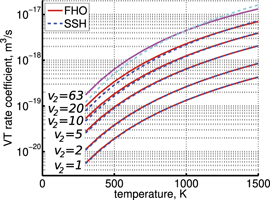
Figure 3. Rate coefficients of the process (22) taken from the set of FHO calculations [19, 45, 46] (solid lines) compared with the coefficients calculated according to the SSH theory [43].
Download figure:
Standard image High-resolution imageThe FHO model also allows to calculate the probabilities of multi-quantum transitions which are not accounted for in first order perturbation theories. Comparison between the rate coefficients of the single-quantum transitions (22) and the corresponding two-quantum rates in the data set [46] shows that at room temperature T = 300 K the two-quantum transitions are always by more than a factor 100 less probable. The importance of multi-quantum transitions is increased at higher T. However, the ratio  —where R1−q
is the rate of a single-quantum transition, and R2−q
is the rate of the two-quantum transition from the same v2—stays
—where R1−q
is the rate of a single-quantum transition, and R2−q
is the rate of the two-quantum transition from the same v2—stays  10 at T ⩽ 1000 K even for the largest v2 = 63 (
 5 at T ⩽ 1500 K). With decreasing v2 the ratio
  is increased.
For transitions other than (3), in particular for VV transfer, the difference between FHO and SSH scalings can be much large. As has been shown above, at T < 2000 K those other transitions are relatively unimportant for thermal excitation of vibrational energy. At the same time, the inter-mode and VV transitions are the processes which govern the fast energy exchange between different kinds of vibrational modes and bring them to the Boltzmann distribution with single temperature Tvibr. Although the absolute values of their coefficients are adjusted to experimental data the SSH scaling can lead to very inaccurate values for high excited states. Nevertheless, as long as those processes in the model are fast enough this inaccuracy must not have large impact on the final result. Strong coupling between different types of vibrations in the two-modes simulations agrees with the fact that in shock tube experiments only one or two very close relaxation times were detected [15, 22].
5. Model system 2: 'thermal dissociation'
The 'thermal dissociation' test serves as experimental check of the calculation of dissociation rate in the vibrational kinetics model. The simulations are performed for conditions of temperature equilibrium—translational–rotational temperature T is equal to vibrational temperature Tvibr. Their results are compared with the dissociation rates measured is shock tube experiments. Behind a shock front vibrational relaxation is much faster than the dissociation, and the assumption that this latter takes place under T = Tvibr conditions is valid. The most reliable experimental data for the speed of reaction CO2 + M → CO + O + M are available for CO2 diluted in Ar. Therefore, the first benchmark here is made for M = Ar rather than for M = CO2 which will be discussed later. The experimental data of [36, 47] are used which were obtained for molar fraction of CO2 in Ar in the range from 10−5 to 10−2.
A comparison of the model with [36, 47] was already shown in the previous paper [21], see section 3.1 and figure 4 there. However, in [21] M = Ar was modelled by M = CO2 with disabled VV transitions. Here the benchmark of [21] is improved by removing that inconsistency. The vibrational transitions of CO2 in collisions with Ar which are taken into account in the present model are listed in table 2. They are added to the transitions between CO2 molecules, table 1 in [21]. The process tags in the first column of table 2 correspond to the notation of [21].

Figure 4. Rate coefficient of the process CO2 + Ar → CO + O + Ar in conditions of temperature equilibrium T = Tvibr. 'Eremin 1997' and 'Burmeister 1990' are the experimental data [36, 47] respectively. Solid lines are the results of the model calculations, see section 5, with two different  decay rates
  and
and  . Dashed lines show the estimated range of uncertainty of the experimental data, equation (23).
Download figure:
Standard image High-resolution imageTable 2. Vibrational transitions of CO2 in collisions with Ar. Same notation as in [21].
| V1 | CO2[vs, va] + Ar ⇆ CO2[vs − 1, va] + Ar |
| V2a | CO2[vs, va] + Ar ⇆ CO2[vs + 3, va − 1] + Ar |
| V2b | CO2[vs, va] + Ar ⇆ CO2[vs + 2, va − 1] + Ar |
The rate coefficients of process V1 are based on the shock tube data of [15]. The relaxation times measured in [15] are in a good agreement with independent measurements of [48]. In [15] vibrational relaxation in pure CO2 and in Ar/CO2 mixture with 10% molar fraction of CO2 was investigated. To reconstruct the rate R10 of (6) with M = Ar  it is assumed that the measured relaxation time τ of the mixture can be expressed as:
where  is the energy relaxation rate coefficient in terms of equation (16) for the corresponding type of 2nd particles M, n is the total number density of Ar and CO2 (the density which determines the total pressure), c is the concentration—molar fraction—of CO2 in the mixture.
  is reconstructed using the data of the pure CO2 experiment in the same paper [15]. After that the
  is found by applying equation (10) with
  . The resulting least square fit is:

In this section in equations for rate coefficients the temperature T is always in Kelvin, and the resulting rate coefficients are in m3 s−1.
The rate coefficients of the processes V2 (see table 2) are calculated in exactly same way as it was done for M = CO2 in [21], see section 2.1 there. The absolute values of the basis rate coefficients for the lowest vibrationally excited states are obtained from the experimental decay rate of the state  . The SSH theory calculations are only used to find the branching ratios. The rate coefficients RV2 of the
  decay determined by laser diagnostics are taken from [49, 50]. The experimental data in [49, 50] are only available for T up to 1000 K, and for the benchmark in question they have to be extrapolated up to 4500 K. The rate coefficient
  had to be extrapolated to high T as well, but for the process V1 this is a smaller issue because: (i) the data are available for T up to 2600 K; (ii) this process was found to be less important for thermal dissociation than the group of processes V2. The small systematic difference between the two references [49, 50] gets significant when they are extrapolated to high T. Therefore, two cases are considered. The decay rate coefficient
  which is the least square fit of the data of [50], and
  which is the fit of [49]:


Calculation of the transition rate coefficients of individual combined states applying SSH scaling is described in detail in [21], section 2.1 there, and in [39]. The only difference is that the reduced mass μ and the characteristic interaction length a−1 must be taken for the pair CO2 + Ar.
The consistency of the final CO2/Ar vibrational kinetics model and the relaxation data of [15] is checked by the same 'behind a shock front' test as in section 4. The test with 10% CO2 in CO2/Ar mixture was performed for the temperatures which correspond exactly to the experimental points of [15]. The time trace  calculated for each experimental case is compared with exponential function (13) where τ is the experimental relaxation time for that temperature point. The maximum relative difference defined by (14) is 17%. As it was seen in section 4 one would expect that at high T the excitation of vibrational energy is not dominated by the processes V1, and R10 calculated by equation (10) is not valid anymore. Hence, the relatively good agreement at the highest T is to some extent a coincidence. Although for M = Ar even in the case with the highest T = 2600 K the channel V1 is still responsible for more than 60% of vibrational energy gain, and (10) is still valid to a certain degree of accuracy.
The results of the 'thermal dissociation' simulations with the updated CO2/Ar model are compared with experimental data [36, 47] in figure 4. The rate coefficients Rdiss are calculated by a least square fit of the time trace  with the function
  , where
  is the number density of CO2 molecules as a function of time t and n0 is the initial total number density of Ar and CO2. It was already shown in the previous work [21] that the calculated Rdiss does not explicitly depend on initial pressure (or on n0). Those tests were not repeated here, all calculations are performed for the nominal pressure 1 bar. The results in figure 4 are all obtained with c = 10−4. Only a little variation in the results was seen when c is increased. The maximum relative difference between the solutions obtained with c = 10−4 and c = 10−2 is 36%, and the relative difference of the solutions obtained with c = 10−4 and c = 10−3 is always smaller than 4%.
As one can see in figure 4 the difference between the simulations made with  and
and  is not large. In both cases at temperatures below 3000...3500 K the model tends to underestimate the rate of dissociation, and at higher temperatures tends to overestimate it. As it was already discussed above in section 3 in the simulations the effective transition probabilities calculated by the SSH theory scalings are always constrained by the prescribed upper boundary
  . As it is shown in figure 4 reducing
  from its nominal value 1 to 0.1 slightly improves the agreement at high temperatures. The dashed lines in figure 4 give the estimated uncertainty of the experimental data [36, 47] provided by the least square fit:
where 0.54 is the standard deviation of residuals. Formally the numerical results obtained with  = 0.1 are almost within this uncertainty. Nevertheless, the calculated dissociation rate apparently grows steeper with temperature than in the experiments. This discrepancy is likely a consequence of the oversimplified way in which the method of 'unstable states' applied in the model to simulate the dissociation reflects the real two-step process as discussed in section 3. The fact that the steepness, hence, effective activation energy, is overestimated by the model speaks in favor of the hypothesis proposed in [41] that the speed of dissociation is also constrained by the speed of the singlet-triplet transition and kinetics of subsequent vibrational excitation of the electronic state 3
B2.
= 0.1 are almost within this uncertainty. Nevertheless, the calculated dissociation rate apparently grows steeper with temperature than in the experiments. This discrepancy is likely a consequence of the oversimplified way in which the method of 'unstable states' applied in the model to simulate the dissociation reflects the real two-step process as discussed in section 3. The fact that the steepness, hence, effective activation energy, is overestimated by the model speaks in favor of the hypothesis proposed in [41] that the speed of dissociation is also constrained by the speed of the singlet-triplet transition and kinetics of subsequent vibrational excitation of the electronic state 3
B2.
In CO2 heavily diluted in Ar VV transitions are effectively disabled and are not involved in the benchmark. In order to test the whole model the rates of dissociation in pure CO2 have to be compared. Opposite to M = Ar there are no direct experimental data for M = CO2. There are two main reasons for that. First is that when processing the results of shock tube experiments there is no straightforward way to separate the primary process CO2 + M → CO + O + M from the oxygen exchange reaction CO2 + O → CO + O2. Second is that the reconstruction of the flow parameters in molecular gases is less certain and more error prone than in atomic gases. Because of that the rate coefficients of the process CO2 + M → CO + O + M with M = CO2 which can be found in the literature are those for M = Ar multiplied by an enhancement factor. This latter is estimated roughly on the basis of experimental data and its value varies from 2.5 to 11 depending on the (literature) source. In figure 5 the model calculations are compared with the fits of dissociation rate coefficients obtained by this method taken from two data reviews [51, 52].
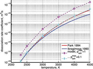
Figure 5. Rate coefficient of the process CO2 + M → CO + O + M, M = CO2 in conditions of temperature equilibrium T = Tvibr. 'Ibragimova 1990' and 'Park 1994' are the fits from the data reviews [51, 52] respectively. Dashed lines are the results of the model calculations with values of the parameter  indicated in the legend.
Download figure:
Standard image High-resolution imageOne can see that the reference model overestimates the literature data by an order of magnitude. Good agreement can only be achieved with reduced  . (Agreement with the data from [52] in figure 5 appears to be exact in this case, but this is coincidence). The results are found to be much less sensitive with respect to the parameter
  (see section 3). Its increase up to
  = 10 leads to only a very moderate increase of the rate coefficient, and its decrease down to
  = 10−2 does not lead to its reduction. Unless
  is much larger than 10 the VV-transitions between asymmetric modes dominate the transitions to unstable states and thus the rate of dissociation. The fact that the result is sensitive with respect to reduction of
  is manifestation of the general shortcoming of the 1st order perturbation theories which was already discussed in section 3. In the microwave discharge studies in section 6 below the
  = 0.1 case is always part of sensitivity tests. Proper solution of this issue would be application of the FHO model [19, 35] instead of SSH at least for the VV-transitions between asymmetric states.
The benchmark discussed in this section still can be seen at best only as a partial validation of the model because the temperatures T > 2000 K are not in the range relevant for investigating the non-equilibrium vibrational dissociation which is the main goal of the present work. Nevertheless, this test shows that despite its very approximate nature especially for high excited states the applied vibrational kinetics model is capable of producing the correct orders of magnitude of the CO2 dissociation rate.
6. Model system 3: 'microwave sustained plasmas'
The vibrational kinetics model [21] calibrated, verified and partially validated as described in the two previous sections has been applied to study the onset of the non-equilibrium vibrational dissociation of CO2 in microwave gas discharges. To simulate the electron impact excitation of vibrational states a model system similar to that of [21] has been adopted with one important modification. Instead of degree of ionization the total specific (volumetric) input power Q into electrons is prescribed and fixed in a model run. In practice this means that the electron density ne is calculated from the power balance:

where ni
is the number density of the excited state i,  is the total rate coefficient of all the electron impact processes which transfer the species i into species k, and
  is the energy spend on average by electrons in each transformation from i to k.
The term Q only includes vibrational excitations and does not include other types of the electron processes such as direct electron impact dissociation or ionization. This approximation is applicable when the electron kinetic energy goes predominantly into production of vibrationally excited states. In weakly ionized plasmas the electron energy distribution function (EEDF) as well as the breakdown of electron energy over different channels is determined by reduced field E/n (see e.g. [11] or [53]) where E is the strength of electric field, and n in the case in question is the number density of CO2 molecules. Numerical calculations [11–13] had shown that for CO2 there is a certain range of E/n around 10 Td—approximately between 5 Td and 50 Td—in which most of the electron energy is indeed spent on the excitation of vibrational states. The order of magnitude of E/n indicated above is typical for the microwave sustained plasmas [54, 55]. Hence, the model system considered here is relevant for the conditions of microwave discharges.
The rate coefficients  are calculated assuming Maxwellian EEDF. This assumption is shown to be approximately valid in microwave plasmas for the processes for which the high energy tail of EEDF is of minor importance, see [56–58]. A more accurate calculation of EEDF was considered to be superfluous since no excited state resolved data are readily available for the electron impact transitions anyway, thus, only a very basic model of those processes is applied. Only one-quantum transitions are taken into account, and same rate coefficients are applied for all excited states, see [21]. The range of reduced field 5 Td ≲ E/n ≲ 50 Td corresponds to the average electron energies of the order of 1 eV [11, 12]. Therefore, electron temperature Te = 1 eV is assumed in the reference simulations here. The effect of variation of Te near this value was found to be very small, see below.
Applicability of the model to gas discharge conditions—although not exactly to microwave plasmas—is checked by simulations performed for the pulsed glow discharge experiment reported in [59]. Only pure CO2 is included in the model. Therefore, as a test case the 'single pulse' experiment presented in figure 7(b) of [59] is taken in which the off-time is long enough to purge the gas from CO and O2 produced due to electron impact processes during the discharge. The duration of the pulse is 5 ms. The pulse voltage is 1.5 kV, discharge current is 50 mA—total discharge power 75 W. The length of the plasma is approximately estimated to be equal to the distance between electrodes—17 cm, and the plasma diameter is the diameter of the discharge tube—2 cm. This yields specific input power 1.4 × 10⁶ W m−3. The gas pressure is 6.7 mbar. At the beginning of discharge when the gas temperature Tg is around 300 K the reduced field is E/n = 55 Td. According to [11, 12] for this value of E/n 70%...80% of input power goes into vibrational excitations. Therefore, in the calculations the specific power which goes into vibrational states is set to Q = 106 W m−3. The electron temperature for the value of E/n above is set to Te = 1.5 eV according to [11].
To reflect the gas heating in the model a time-profile of translational–rotational temperature T is prescribed according to the time dependency of Tg shown in [59] (figure 7(b)). The master equations are solved in constant pressure form. The dissociation of CO2 from high vibrational states in the conditions in question is found to be zero. The results of simulations are shown in figure 6 as time evolution of the temperatures of symmetric Ts and asymmetric Ta modes. The profile of Tg and the definitions of Ts and Ta can be found in appendix
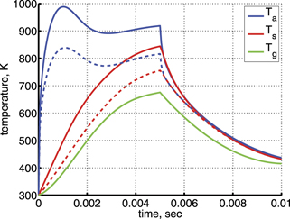
Figure 6. Results of calculations for conditions of the 'single pulse' experiment of [59], pressure 6.7 mbar, plasma current 50 mA. The symmetric and asymmetric temperatures Ts and Ta are defined in appendix
Download figure:
Standard image High-resolution imageAt least part of this discrepancy can be ascribed to the lack of self consistency in the present model. As Tg is increased at constant pressure the reduced field E/n is increased too. Thus, the fraction of input power which goes into vibrationally excited states has to get smaller, see [11, 12], and Q has to be reduced as well. Indeed, calculations with Q = 5 × 10⁵ W m−3 shown in figure 6 by dashed lines yield temperatures in the end of discharge phase which are closer to the experiment. The parameters  and
and  of the two-modes model, see section 3, were found to have very weak influence on the outcome of the test. Variation of the parameter
  from 10−2 to 10, and reduction of
  to 0.1 have found not to affect the results shown in figure 6. Two more factors not included in the simulations may be responsible for the remaining disagreement with experiment besides the vibrational kinetics itself. First are the losses of vibrational energy due to spontaneous emission which can become significant at low pressures. Second is the hydrodynamics of the gas expending due to heating approximated here by the constant pressure assumption.
The set of master equations solved by the model in the discharge zone Q > 0 can be written in the same form as (21) with the electron excitation term added:
The following transformation applies when Q = const. Equation (24) is substituted for ne, the number densities are replaced by concentrations ck
: nk
= ck
n0. Finally, specific energy input (SEI) per one initial molecule = Qt/n0 is introduced, bringing the equations above into the form:

As one can see from (25) for the constant T and Te the solution expressed in terms of ci
and depends only on the parameter  . This is exactly same parameter as in the approximate threshold criterion (17) in section 2.2.
The outcomes of the model calculations for selected fixed temperatures T are shown in figure 7. The results are presented in terms of  and the 'process rate' χ defined as the fraction of initial CO2 molecules which dissociate in the process CO2 → CO + O. For all model runs this quantity is taken at the time instants which correspond to = 3 eV:

Conversion in the afterglow (Q = 0) is not taken into account since in the previous work [21] the conversion on that phase was found to be insignificant. The chosen final value of is close to the net enthalpy change of the total process CO2 → CO +  O2, ΔHf = 2.9 eV [40] which is the ideal cost of producing one CO molecule. That is, which is larger than that value will lead to inevitable losses of energy not into the target process even at 100% conversion of CO2 into CO and is therefore not considered.
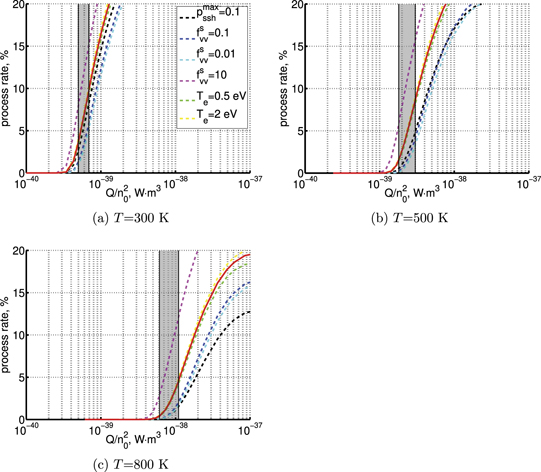
Figure 7. 'Process rate' χ defined by (26) as a function of parameter  , see equation (25), calculated by the two-modes model [21] for fixed translational–rotational temperatures T. Solid line is the reference model, dashed lines are the simulations with uncertain parameters varied, see sections 3 and 6. Shaded rectangles is the approximate calculation of
  , section 6.1.
Download figure:
Standard image High-resolution imageThe CO2 kinetics model applied for the simulations here is incomplete in terms of chemistry—it does not include the secondary processes with O-atoms and reverse reactions. Also, interaction of CO2 with reaction products CO, O2, O is not taken into account. Therefore, the calculated χ is not expected to be a quantitatively correct prediction, but rather an indicator that the process has been started. At the same time, the model can be considered as valid in the vicinity of the threshold values of  there the total CO2 conversion is yet low and the influence of products on the primary dissociation process is yet small. That is, the determination of the
  threshold above which the efficient dissociation from high vibrational states can start is the main result of the simulations, not the absolute values of χ at higher
  .
.
All the simulations presented in figure 7 were performed technically for the nominal pressure p = 100 mbar. To confirm that, as suggested by (25), there is no explicit pressure dependence the calculations were repeated with different values of p. The relative differences of χ calculated with p = 50 mbar and p = 200 mbar and those with p = 100 mbar for the same values of  (only χ > 0.1% are taken into account) are found to be always
  0.7%.
0.7%.
The solid lines in figure 7 present the solutions obtained with the reference model, and the dashed lines are the results of the simulations where the model uncertainties are evaluated. In particular, the impact of the parameters  and
and  described in section 3. The effect of reducing the parameter
  from 1 to 0.1 is visible although relatively small for T = 300 K, but tend to increase at higher T. For the parameter
  the values 10−2, 10−1 and 10 were tested. One can see a relatively large modification of the solution, especially when
  is increased. At the same time, one can also say that both the variations of
  and
and  —although they have substantial impact on the steepness of the χ increase with increased
  —have a very limited effect on the threshold value of this parameter. Finally, the effect of changing the electron temperature Te was also investigated. In the reference model (Te = 1 eV) 69%...81% of Q is deposited into asymmetric modes va. Two model runs have been added with Te = 0.5 eV and 2 eV. In the first case the fraction of Q which goes into asymmetric modes is slightly increased up to 80%...92%, in the second case it is reduced down to 57%...70%. As one can see in figure 7 those variations have negligible impact on the solution.
6.1. Process threshold 

In this subsection the results of the vibrational kinetics simulations above are compared with the simple formula (17). First, it has to verified that equation (16) with RVT determined from gas dynamic experiments is approximately valid for the microwave discharge conditions as well. For that the magnitude of the term QVT as it appears in the simulations is compared directly with QVT calculated by (16). Examples of this comparison are shown in figure 8. Instead of Evibr the more illustrative quantity Tvibr is used. To translate the simulated Evibr into Tvibr equations (A.2) and (A.3) from [21] are used, Evibr in (16) is calculated as a function of Tvibr by applying (12). The  in (16) is calculated by (20), with R10 taken from [28]. To remind, the two-modes model [21] which has been applied for the simulations here is adjusted to match the experimental rates of vibrational relaxation which correspond to exactly this choice of
  .
.
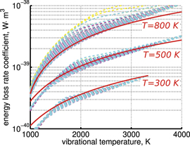
Figure 8. Rate of vibrational energy losses QVT, see (15), divided by nM
n. Solid line is the result of the approximate formula (16), dashed lines are  taken from numerical simulations of section 6. Only modelling runs with the process rate χ < 12% are plotted.
Download figure:
Standard image High-resolution imageOne can see in figure 8 that the agreement is relatively good. This statement is quantified by examining the ratio of  taken from the simulations and
  calculated with (16). For T = 300...600 K this ratio always lies between 0.4 and 1.5. These maximum and minimum are taken over the all modelling runs including those with varied Te,
  and
and  (only points with Tvibr > T + 100 K are taken into account). For higher T the upper boundary (maximum) of the ratio above is increased: up to 2.4 for T = 800 K and up to 3.4 for T = 1000 K. Nonetheless, even in those cases (16) can always be taken as a good order of magnitude estimate. This is an expected result since vibrational distribution function of the lower vibrational levels in the gas discharge simulations was found to be close to Boltzmann, see an example in [21]. The populations of the upper levels near the dissociation limit deviate strongly from the Boltzmann distribution. However, since their absolute values are relatively small the high energy tail they form has no overwhelming impact on the total energy exchange rate.
The critical  (or
(or  ) which enters (17) can be formally determined from the condition that at this
  the dissociation term Qdiss starts to be comparable with QVT, e.g. by taking
  . Unlike QVT there is no simple way of calculating
  , in particular because the dissociation proceeds from the non-Boltzmann high energy tail of vibrational distribution. Therefore, the determination of
  relies on the results of numerical simulations. The model uncertainties lead to a relatively large scattering of that quantity, but, as it will be seen below, this scattering has only minor impact on the final result.
The ratio  obtained in the simulations is plotted for selected T in figure 9. The maximum and minimum of Tvibr which correspond to
  for each T are quoted in table 3. The numbers are rounded off because no high accuracy is required here. The corresponding values of
  are obtained by applying equation (17) with
  calculated using (12). One can see that the variation of
  caused by the uncertainty of
  is not large. The increase of
  with increased T is mainly due to the increase of
  rather than due to the term in [...] in (17).
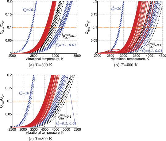
Figure 9. Ratio of the Qdiss and QVT terms, equation (15), as function of Tvibr in numerical simulations of section 6. Solid lines correspond to the reference model with different values of Te. Dashed lines are the cases with  = 0.1 and
  = 10−2, 10−1, 10. Only modelling runs with the process rate χ < 25% are plotted.
Download figure:
Standard image High-resolution imageTable 3. Semi-empiric estimate of the critical value of  , see section 6.1.
| T, (K) |
 , (K) , (K) |
 , (W m3) , (W m3) |
 , , 
|
|---|---|---|---|
| 300 | 2500..3200 | (5..7) × 10−40 | 30..40 |
| 500 | 2900..4300 | (2..3) × 10−39 | 40..60 |
| 800 | 3300..5000 | (6..11) × 10−39 | 50..90 |
| 1200 | 3700..5500 | (2..3) × 10−38 | 60..100 |
The range of  from table 3 is shown as shaded rectangles in figure 7. The agreement with the process threshold as it appears in the results of the simulation runs is very good. That is, for practical purposes the accuracy of the formula (17) together with the approximate values of
  provided in table 3 in determining the process threshold is notworse than the accuracy of a complicated vibrational kinetics model. The estimated magnitude of
  3000...4000 K agrees with the temperatures at which efficient dissociation is observed experimentally under temperature equilibrium T = Tvibr conditions, see figure 4.
7. Discussion
Besides the restrictions discussed above straightforward energetic constrains on SEI have to be fulfilled for efficient dissociation of CO2. SEI is the specific energy input per initial CO2 molecule. SEI has to be at least larger than the energy per molecule which corresponds to the target vibrational temperature Tvibr: e.g. for Tvibr = 3000 K this is 0.8 eV. At the same time, as it was already mentioned in section 6 SEI cannot be allowed to be much larger than the net enthalpy change of the net process CO2 → CO +  O2, ΔHf = 2.9 eV [40].
To summarize, for the non-equilibrium vibrational dissociation at low T to be possible at least three conditions have to be fulfilled simultaneously. SEI and the reduced field E/n must lie in a certain—relatively narrow—range, and the parameter  must be larger than some critical value. As it was shown in section 6.1 the semi-empiric estimate yields
  = 6 × 10−40 W m3 (averaged) at T = 300 K. The numerical experiments suggest that within variation of the modelling result no non-equilibrium vibrational process is possible when
  . At the same time,
  merely means that the non-equilibrium process starts to be measurable. In this regime still most of the power Q goes directly into translational–rotational modes. Efficient conversion of CO2 into CO by the non-equilibrium process can be expected only when Q is further increased, possibly by a factor 5–10, that is, when
  is larger than
  within an order of magnitude.
The critical  calculated theoretically can be compared with the peak values observed in real microwave plasmas. In order to do that it is more convenient to replace n0 with the pressure p = n0
T (T in energy units):
calculated theoretically can be compared with the peak values observed in real microwave plasmas. In order to do that it is more convenient to replace n0 with the pressure p = n0
T (T in energy units):

The corresponding values of  can be found in the last column of table 3. Despite T2 in the denominator the
  increases with increased T. This is mainly because
  in (17) grows faster than ∼T2.
Very accurate reconstructions of the profiles of the volumetric specific power Q have been performed for the surfaguide CO2 plasma conversion experiments at the DIFFER Institute. In figure 10 peak values of Q/p2 taken from the publications [55, 60, 61] are shown. The largest set of data is taken from Wolf 2020 [60], from figure 4 there. Those data represent the experiments with power absorbed in plasma varying from 435 to 1300 W and flow rate 12 slm (standard liter per minute). The parameters correspond to global SEI = 0.5...1.5 eV. The data from Wolf 2020 are supplemented by the pressure scan from Viegas 2020 [55] (figure 3 there): input power 1400 W, flow rate 18 slm, global SEI = 1.1 eV. Two more points have been added from the recent publication Viegas 2021 [61] where the accuracy of the reconstruction of Q was improved. The peak values of Q are taken from figures 9 and 11 in [61] which present respectively the experiments with pressure 110 mbar, power 950 W, flow rate 9 slm (SEI = 1.5 eV), and 150 mbar, 860 W, 12 slm (SEI = 1 eV).
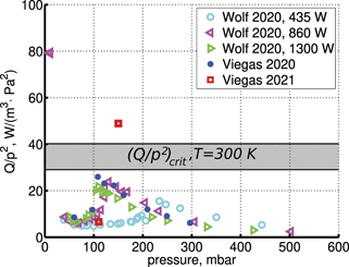
Figure 10. Peak values of the parameter Q/p2 for selection of surfaguide experiments [55, 60, 61], see section 7 for description. Shaded area is the critical value for T = 300 K, see table 3.
Download figure:
Standard image High-resolution image
In all those experiments T > 2000 K are observed, and the measured CO2 conversion is explainable by thermal quenching mechanism. At the same time, one can see that almost all Q/p2 in figure 10 lie below even the room temperature  . That is, from the point of view of the theory of the present work no non-equilibrium vibrational dissociation process was possible in those experiments, and most of the absorbed microwave power should indeed eventually go into the gas heating. Two exceptions are the p = 150 mbar point from Viegas 2021 and the lowest pressure p = 10 mbar point from Wolf 2020. In the first case Q/p2 is only marginally larger than
  for T = 300 K. In the second case Q/p2 is by more than a factor 2 larger than
  . The theory does not exclude that in this case the non-equilibrium process could start at T = 300 K, although with yet low process rate, see figure 7(a). In the experiment strong gas heating was observed in this case same as in other cases, with peak temperature 2300 K. So a weak non-equilibrium effect even if it occurred in the beginning could be masked by subsequent heating of the gas and transition to thermal process.
For the IPP Garching plasma torch experiment [10] no detailed reconstructions of the Q profiles have been published. In contracting mode at high pressures the specific input power can be approximately calculated from the estimated plasma diameter dpl and length Lpl presented in figures 9(b) and 11(b) of [10]. Measurements for the experiments with the following parameters are shown there: pressure 200, 500, 900 mbar, flow rate 20 slm, absorbed power from 900 to 2700 W, global SEI from 0.6 to 1.9 eV. The boundary of the plasma region is approximately defined as the region where the intensity of radiation is above 15% of its maximum. Dividing the absorbed power by the plasma volume calculated as  gives Q/p2 which are always smaller than 6 W (m−
3 Pa−
2). That is, always well below
gives Q/p2 which are always smaller than 6 W (m−
3 Pa−
2). That is, always well below  even at T = 300 K. In homogeneous mode at low pressures before the plasma contracts the extreme assumption that the plasma occupies the whole discharge tube (inner diameter 26 mm) leads to the following numbers. For Lpl = 40 mm (approximately the high of the waveguide) and the largest absorbed power 2700 W Q = 1.3 × 10⁸ W m−3. For the smallest reported pressure 20 mbar that yields Q/p2 = 32 W (m−
3 Pa−
2) which does not exceed the critical value. One has to keep in mind that the local peak values can be higher than the averaged ones.
even at T = 300 K. In homogeneous mode at low pressures before the plasma contracts the extreme assumption that the plasma occupies the whole discharge tube (inner diameter 26 mm) leads to the following numbers. For Lpl = 40 mm (approximately the high of the waveguide) and the largest absorbed power 2700 W Q = 1.3 × 10⁸ W m−3. For the smallest reported pressure 20 mbar that yields Q/p2 = 32 W (m−
3 Pa−
2) which does not exceed the critical value. One has to keep in mind that the local peak values can be higher than the averaged ones.
To conclude, for the selection of experiments reviewed here the parameter Q/p2 in most cases formally smaller than the theoretical  . This agrees with the fact that no significant dissociation due to the non-equilibrium vibrational process could be identified in those experiments. Exceptions are the experiments with very low pressure p ≲ 20 bar where Q/p2 can be marginally higher than the room temperature critical value. In particular under low pressure conditions the reduced field E/n constrain may be more critical than the one due to the parameter Q/p2. At low pressures the reduced field E/n may become too large and out of the optimal range for preferential excitation of vibrational states. Besides that, at very low pressures one more issue occurs which was left entirely out of the scope of the present work. Here total opacity for spontaneous emission from vibrational levels was always implicitly assumed. At sufficiently low gas density the radiative losses of vibrational energy may become significant. Proper account of them would require solving a radiative transport problem. Analysis of glow discharge experiments in [62] indicated that at p = 5 Torr spontaneous emission from asymmetric vibrational states could already have non-negligible impact on their population.
8. Summary and outlook
In this paper activation of the non-equilibrium vibrational dissociation of CO2 at low translational–rotational temperatures T in microwave gas discharges is investigated by means of semi-empiric and computational models. A governing parameter  has been introduced, where Q is the volumetric specific power coupled into vibrational modes, and n0 is the initial number density of CO2. It has been shown that the non-equilibrium process can only be triggered when
  exceeds some critical (threshold) value. To back and extend the semi-analytic results the approximate two-modes state-to-state model of CO2 vibrational kinetics [21] is applied.
The model is calibrated and benchmarked to match at T ⩽ 1500 K the characteristic vibrational relaxation times measured in shock tube and acoustic experiments [15, 22, 28]. The dissociation process CO2 + M → CO + O + M is included in the model via introduction of unstable states whose vibrational energy is larger than prescribed dissociation limit. This approach is partially validated by comparing with shock tube measurements [36, 47] of dissociation rates of CO2 diluted in M = Ar at T > 2000 K, as well as with literature data [51, 52] on dissociation in M = CO2. In this latter case good agreement could only be achieved with artificial upper limit applied to transition probabilities calculated by the SSH theory. This result emphasizes drawbacks of the first order perturbation theories and strongly supports the application of non-perturbative models such as FHO [19, 35] despite their higher complexity. Applicability of the model for the non-equilibrium gas discharge conditions with T < 1000 K has been checked by comparing with the pulsed glow discharge experiment [59]. The model is shown to reproduce qualitatively the time evolution of the temperatures of symmetric and asymmetric vibrational modes, although there is no accurate quantitative much with the experimental results.
A series of 0D two-modes simulations has been performed for a model system which mimics vibrational excitation of CO2 in microwave discharges. In agreement with the analytic consideration the simulations indicate a rapid increase of the rate of the process CO2 → CO + O with increased  when this parameter exceeds some critical value. The solutions are found to be sensitive with respect to variation of the uncertain model parameters. However, the position of the process threshold
  as it appears in the simulation results is relatively stable. A simple estimate of
  based on the experimental rates of vibrational relaxation agrees well with the modelling results. At T = 300 K this estimate provides
  = 6 × 10−40 W m3 or
  = 35 W (m−3 Pa−2) (averaged), where p is the gas pressure. In the temperature range from 300 to 1200 K the
  is shown to always increase with increased T. Analysis of selected experimental publications [10, 55, 60, 61] has shown that in the real microwave discharges the parameter Q/p2 is typically below the estimated critical value. At best the Q/p2 has found to be only marginally (within a factor 2–3 at maximum) above the room temperature
  at very low pressures p ≲ 20 mbar. This observation agrees with the fact that no significant CO2 conversion due to the non-equilibrium vibrational dissociation in the experiments in questions is reported.
The state-to-state model used in the present paper is applicable only near the  threshold where the rate of conversion via the primary process CO2 → CO + O is not yet too high. In order to further extend its applicability the secondary reactions with oxygen, reverse processes, reaction products and their influence on vibrational kinetics must be added. It can be expected that such extensions will not significantly affect the position of
  , but they might have a large impact on the steepness of the conversion rate growth with increased
  .
.
Adding CO to the model can be seen as a purely technical matter since all the data and models for calculation of the transition rate coefficients are readily available. Adding the oxygen chemistry, on the opposite, can face large difficulties because of the exchange reaction CO2 + O → CO + O2. Too little is known about the influence of vibrational non-equilibrium on that process. To which exactly extent vibrational excitation of CO2 speeds up this reaction? The process has a relatively low enthalpy change, where the vibrational energy of CO2 will then go? Will it go into vibrational energy of the products or into their translational–rotational energy? Those questions have no definitive answers. The energy efficiency of the overall conversion process CO2 → CO +  O2 triggered by the non-equilibrium dissociation can be larger than 53% only if the reaction CO2 + O → CO + O2 is faster than the three-body recombination O + O + M → O2 + M, and if vibrational energy of CO2 which takes part in the former goes predominantly into the products vibrational energy.
It is unlikely that all the unknowns will be resolved soon. Thus, it is unlikely that models which correctly predict the efficiency of the overall non-equilibrium CO2 conversion process can be developed in the near future. At the same time, accurate model predictions of the conditions at which the non-equilibrium process could be triggered are realistic. In particular, the models for CO2/CO/O2/O mixtures without exchange reaction CO2 + O → CO + O2 are feasible. Computational models of that kind may help to find the parameters under which the low T non-equilibrium process can be obtained and studied experimentally. The  criterion alone introduced in the present work only makes sense when most of the power absorbed in plasma goes into excitation of vibrational states, that is, only for a certain range of reduced field E/n. To account for this constrain automatically it is mandatory that a model includes detailed electron kinetics. Models which couple self-consistently the electron kinetics and the CO2 vibrational kinetics and chemistry do exist [13, 57, 58]. Their main issue is that the cross sections of the electron processes with vibrational states of CO2 are not known to a high degree of accuracy.
Data availability statement
The data that support the findings of this study are openly available at the following URL/DOI: https://doi.org/10.26165/JUELICH-DATA/IHO9NP. The up-to-date source code of the numerical model (Fortran) can be found at the following link: https://jugit.fz-juelich.de/reacflow/co2-20.
Appendix A.: Derivation of vibrational relaxation equation for CO2
Derivation of the equation which describes thermal excitation of vibrational energy in diatomic molecules can be found in [14], chapter 19. Here the derivation of [14] is modified for CO2 which has three modes of oscillation v1, v2, v3. The mode v2 is double degenerate and has rotational momentum l:  . It is assumed that the molecules are linear (harmonic) oscillators and their vibrational energy Ev can be expressed as:

Further assumptions are that vibrational–translational (VT) transfer takes place only from the mode  via process (3), and the number of vibrational states is infinite.
Since in the linear oscillator approximation Ev does not depend on l all states with same v2 can be gathered into a combined state. There are v2 + 1 different values of l possible for a fixed v2. The normalized matrix elements X of all possible VT-transitions from the mode  are summarized in [39], see equation (27) there:


The averaged probability p of transition between combined states v2 and v2 − 1 calculated by the first order perturbation theory (SSH) is proportional to:

The sum ∑l is taken over all values of l allowed for the corresponding v2. Same for the transition between combined states v2 and v2 + 1:
Some transitions which appear in the sums are not possible. For example the transition from  to
to  is not possible because this latter state does not exist. Such transitions must not be excluded explicitly from the sums because the formulas for X automatically give zero in those cases.
Taking into account the assumption that only VT-transitions between modes  , process (3), are possible the particle balance equations for the number densities n of the combined vibrational states
  read as follows:

Here k are the transition rates: transition rate coefficients multiplied by the total density of particles M in the process (3). The coefficients k10 and k01 are connected by the detailed balance relation:
Here wj
is the degeneracy of the vibrational level  which is equal to j + 1, and Ej
is its vibrational energy.
which is equal to j + 1, and Ej
is its vibrational energy.
All the other rate coefficients in (A.3) and (A.4), can be connected with k10 using the expressions (A.1), (A.2) and (A.5):


Equations (A.6) and (A.7) are substituted into equations (A.3) and (A.4). For convenience of notation indexes v1, v2, v3 are replaced by i, j, k respectively. The resulting master equations read:

To obtain the energy relaxation equation the (A.8) and (A.9) are multiplied by:

and then their sum over indexes i, j, k is calculated. This sum reads:
The second term in (A.10) equals zero. Indeed, combining the terms without K in the innermost sum yields:
Same for the terms with factor K:
The sum:
is the total specific (per unit volume) vibrational energy; Evibr is the specific vibrational energy per molecule, n is the total number density of molecules. The whole equation (A.10) is reduced to the following form:
Calculation of the first sum of (A.11):
Calculation of the second sum of (A.11):
Substituting the calculated sums back into (A.11) yields:

where:
is the total vibrational energy stored in the mode  , Evibr-2 is its specific value per molecule. Transforming the right-hand side of (A.12) and substituting K, equation (A.5), yields finally:
For n = const. and with k10 replaced by  this equation gives (4) and (5).
Appendix B.: Details of the model of the experiment [59]
For a constant pressure system it is more convenient to write the master equations in terms of total number of particles Ni of each component i rather than their number densities ni :

Here Si is the specific (per unit volume) particle source of the component i and V is the variable volume of the system determined from the equation:

Here the sum ∑ is taken over all components i, T is the translational temperature (in energy units), p is the total pressure. Equation (B.1) is readily translated into equation for ni when one can assume that the total number of particles is conserved, ∑Ni = const. This assumption is valid for the pulsed glow discharge test of section 6 where vibrational temperatures are very low and vibrational dissociation does not take place. In this case substituting Ni = ni V and (B.2) into (B.1), and recalling that p = const. yields:

The dependence of the gas temperature Tg shown in figure 7(b) of [59] from time t is fitted by the function:
where a0 = 300, a1 = 3.479 6276 × 104, a2 = 6.289 9233 × 107, a3 = −1.809 2153 × 1010, a4 = 1.425 3195 × 1012; b0 = 675.767 76, b1 = −1.005 9133 × 105, b2 = 9.708 9841 × 106; tpl = 5 × 10⁻³ sec, t is in seconds, Tg in Kelvin.
The temperatures (in energy units) Ts and Ta are defined as:
where ![${n}_{[{v}_{\mathrm{s}},{v}_{\mathrm{a}}]}$](https://content.cld.iop.org/journals/0963-0252/31/9/094002/revision2/psstac882fieqn212.gif) are the number densities of the corresponding two-modes states, and
are the number densities of the corresponding two-modes states, and ![${E}_{[{v}_{\mathrm{s}},{v}_{\mathrm{a}}]}$](https://content.cld.iop.org/journals/0963-0252/31/9/094002/revision2/psstac882fieqn213.gif) are their vibrational energies (E[0,0] = 0). For the case shown in section 6 the temperatures Ta defined for the first 4 levels [0, va] are equal within relative difference of 3%, the same applies to Ts defined for the first 10 levels [vs, 0].
are their vibrational energies (E[0,0] = 0). For the case shown in section 6 the temperatures Ta defined for the first 4 levels [0, va] are equal within relative difference of 3%, the same applies to Ts defined for the first 10 levels [vs, 0].
Footnotes
- 1