
Abstract
Perkins et al (2012 Phys. Rev. Lett. 109 045001) reported unexpected power losses during high harmonic fast wave (HHFW) heating and current drive in the National Spherical Torus Experiment (NSTX). Recently, Tierens et al (2020 Phys. Plasmas 27 010702) proposed that these losses may be attributable to surface waves on field-aligned plasma filaments, which carry power along the filaments, to be lost at the endpoints where the filaments intersect the limiters. In this work, we show that there is indeed a resonant loss mechanism associated with the excitation of these surface waves, and derive an analytic expression for the power lost to surface wave modes at each filament.
Export citation and abstract BibTeX RIS
1. Introduction
Reportedly [1, 2], during high harmonic fast wave (HHFW) heating and current drive in the edge plasma of the National Spherical Torus Experiment (NSTX), a substantial fraction of the radiofrequency power fails to reach the core plasma. Instead, it flows along field lines and hits the divertors.
Over the years, many explanations for these unexpected losses have been put forward, involving fast waves (FW) [3], slow waves (SW) [4, 5], sheath rectification [6, 7] and parametric decay [8].
Recently, we proposed a mechanism that can explain why such losses are observed on NSTX but not elsewhere [9] (i.e. mainly in conditions with HHFW and small parallel wavenumber ( )). Knowing that small (non-ELM) filaments are plentiful in the NSTX SOL [10, 11], we used an analytic solution for wave scattering at plasma filaments [12], which shows that surface waves on such filaments can be resonantly excited and carry power along the filaments and thus along the field lines. This is more common in the HHFW heating scenarios used in NSTX than in generic ion cyclotron range of frequencies (ICRF) heating scenarios. We hypothesized that the power would be lost due to some endpoint loss mechanism (e.g. sheath rectification, imperfect reflection, surface resistivity) where the filament finally intersects a divertor.
In this work, we quantify the amount of power that is redirected to the surface waves in an idealized case (infinite magnetic field lines) where the end point mechanisms are not present. We follow an approach that should be generic to any resonant surface-wave-like oscillations. The main steps are as follows.
- (a)Derive the resonance condition for surface wave excitation on a given filament. Specifically, find the parallel wavenumber
 at which a resonance occurs for prescribed filament properties (density, radius). Several resonant values may exist.
 - (b)Introduce a causality parameter ν, formally similar to a collision frequency, as explained in [13].
- (c)Calculate the total power dissipated in the filament from step (a), with ν > 0.
- (d)The resulting integrand has Lorentzian terms with peaks at the resonant, growing higher and narrower, but remaining integrable, as ν decreases.
- (e)Take the limit. If the filament is long enough, we show that the asymptotic dissipated power remains finite, independent of ν. We claim that the result is fairly independent of the physical dissipation mechanism described phenomenologically by ν (appendix
A ). - (f)Average the dissipated power over the filament type. Filaments are inherently random structures in terms of density/radius, with each a specific probability to be present at a given time, and a specific resonant value that matches a specific part of the launched spectrum for the incident waves.


This work is organized as follows: in section 2 we analytically perform step (a) for one specific branch of resonant modes relevant in the HHFW regime. In section 3 we derive the power redirected due to this resonant surface wave excitation (steps (b)–(e)). Section 4 contains a discussion of the statistical nature of the filaments and the average power converted per filament (step (f)). An example is given in section 5, and the conclusion is given in section 6.
2. Derivation of the resonance condition
We consider a wave scattering problem much like that discussed in [9, 12]: a cylindrical filament with radius rf
and constant density nf
, in a background plasma with constant density nb
. The filament is along the confining magnetic field, which is along z. The parallel direction (subscript  ) is always along z, parallel to B. The perpendicular direction (subscript
  ) is perpendicular to B. We use a cylindrical coordinate system
  or
or  centered on the filament.
In [9], we identified multiple kinds of conditions under which surface waves exist on the filament. Here, we try to find an approximate analytical expression for the resonance condition for the ones we expect to be physically relevant in the HHFW regime, the ones which occur when  is not much greater than 1.
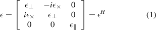
We start by writing the dielectric tensor in the HHFW limit (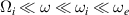 )
)
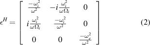
where  ,
,  ,
,  ,
,  , with f the launched wave frequency, and qi
and mi
the ion charge and mass. For simplicity, we assume a single-ion plasma. In the range of plasma parameters of interest for this work, the slow wave is evanescent, and its perpendicular wavevector
, with f the launched wave frequency, and qi
and mi
the ion charge and mass. For simplicity, we assume a single-ion plasma. In the range of plasma parameters of interest for this work, the slow wave is evanescent, and its perpendicular wavevector  is purely imaginary, with imaginary part κ
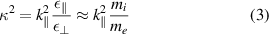
which is conveniently independent of the density, in the HHFW limit. Throughout this work, we will assume without loss of generality that  and κ are positive. Following [14], we introduce a spectral representation of the scattered SW field, in the filament and in the background
with the amplitudes  to be determined. We will see that the poles of
  and
and  are the resonances for which we are looking. Next, we write
  as the gradient of a potential [14]


where  are Bessel functions. This approximation requires that
  is negligible w.r.t.
  , which fails for
  . In practice, ICRF antennas avoid exciting very low
  modes, especially when operating in dipole, which is common. As will be clear soon, only one azimuthal mode can be resonant,
  depending on the the type of filament. Therefore, to simplify the notation in the following we omit the sum over m. For the fast wave, since
  , the perpendicular electric field of the incident FW is nearly constant across the radial scale of the filament. Mathematically, this is equivalent to approximating
  by
by 
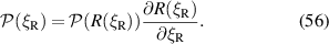
where  is the spectrum of
  of the incident FW launched by the antenna. Thus, the perpendicular component of the solution of the wave equation can be approximated by the perpendicular gradient of the following potential
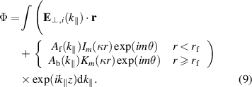
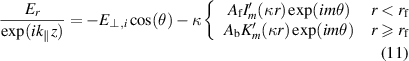
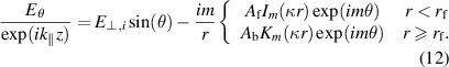
In the spirit of the Born approximation [15], we omit the contribution from the scattered fast wave since it is negligible to the lowest order. Although our approach should remain valid in the case where the scattered fast wave is evanescent, this approximation is especially well-justified in the case where it is propagative: the surface wave cannot radiate energy away from the surface, and thus cannot contain a significant contribution of a propagating fast wave. As a consequence of this approximation, we will see the surface waves on the filament gain energy from the incident fast wave, but we will not see the fast wave lose energy—an approximation that is only really valid in a perturbative regime where at most a small fraction of the incident power is lost to the surface waves. Within these approximations, of the six boundary conditions on the interface [12], only two are not trivially satisfied: the continuity of Φ ( from the fast wave is continuous by assumption since we neglect the scattered fast wave, and the continuity of
  from the scattered slow wave follows from the continuity of Φ) and the continuity of
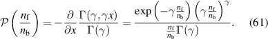
  at the filament surface. These two boundary conditions suffice to constrain the unknown coefficients
  and
and  . The first gives

For the continuity of Dn
, we consider a single  mode, where we may assume without loss of generality that
  points along the x axis, and
  . Then
The matching condition for Dn is

and writing it all out:
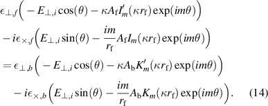
It is clear that only  modes can be excited by the incident FW. Projecting (14) onto
  using
using  ,
, 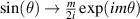 ,
,
where  . The argument of the Bessel functions and their derivatives is from now on assumed to be ξ when not explicitly given. Collecting terms in the unknown amplitudes
  , (15) becomes

where


The solution which obeys both continuity conditions, (10) and (16), is
In the HHFW limit,  and
and  are both proportional to the density. Normalizing everything to the background density (i.e. unless otherwise noted, ωi
and ωe
are calculated from the background density
are both proportional to the density. Normalizing everything to the background density (i.e. unless otherwise noted, ωi
and ωe
are calculated from the background density  ), and using
  and
and  (
( in HHFW),
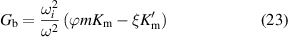
The resonance condition  , where
  and
and  have a pole, becomes
In figure 1 we see  and
and  . To determine the forward or backward nature of these waves, we can solve the resonance condition for ϕ
Figure 2 shows (25) for various values of ϕ. From both theory [16, 17] and experiment [11], we know that filaments with  not much greater than 1 are common, but filaments with much higher
  are rare. It becomes clear that this mechanism is relevant for HHFW (
 ) but not for traditional minority and second harmonic ICRF heating: exciting the surface waves in the latter case requires much higher, hence much rarer,
  .
.
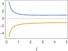
Figure 1. Logarithmic derivative  (blue, always positive) and
  (orange, always negative).
Download figure:
Standard image High-resolution image
Figure 2.
 given by (25), for blob filaments (
 , left) and for hole filaments (
 , right). We show
  on the upper x axis, with
  assuming deuterium plasma and
  cm.
cm.
Download figure:
Standard image High-resolution imageWhile the approximations made in this section may seem extreme, we have previously determined the locations of these resonances within an exact electromagnetic full-wave solution [9]. In figure 3, we see that (25) is indeed a good approximation to the resonances found in that exact full-wave solution, which justifies our approximations. Numerical calculations in [18, 19] and theoretical arguments in [20] also confirm that such resonances exist even for nonidealized filaments.

Figure 3.
 given by (25) as white dashed lines, overlaid on the resonances found in [9] within a full electromagnetic solution for wave scattering at a filament. There is a second set of resonances at the bottom of the figure. These resonances arise when the SW can propagate inside the filament but not in the background [14], but they are not relevant for the rest of this work. The side plots give the wavelengths of the FW and SW, black for propagative, red for evanescent.
Download figure:
Standard image High-resolution image2.1. Blob filaments (R > 1)
 and
and  are all positive while
  is negative (figure 1). Thus, for filaments whose density exceeds that of the background (so-called 'blob filaments', where R > 1), (25) predicts that resonances can only exist at m = 1,
  , and
, and  , where
  is the positive root of
  . From (26),
  for
for  , so the surface waves resonantly excited on blob filaments are forward in the parallel direction.
2.2. Hole filaments (R < 1)
For filaments whose density is below that of the background (so-called 'hole filaments', where R < 1, see [21]), (25) predicts that resonances can only exist at  ,
,  , and
, and  , where ξ0 is the positive root of
  . From (26),
  for
for  , so the surface waves resonantly excited on hole filaments are forward in the parallel direction.
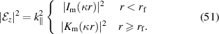
3. Derivation of the filament losses
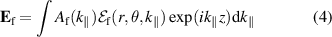
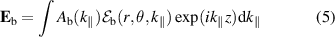
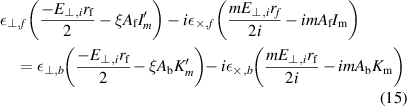
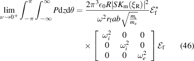
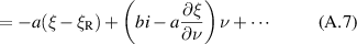
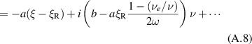
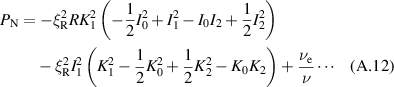
We now introduce the causality parameter ν, formally similar to a collision frequency, in the dielectric tensor

The case where ν plays the role of a physical collision frequency, and the electrons and ions have different collision frequencies, will be treated in appendix  and
and 
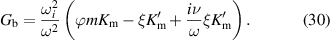
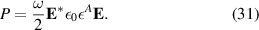
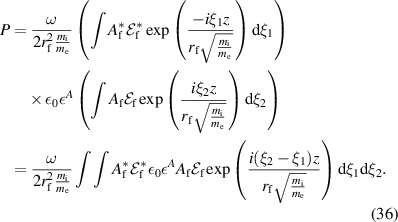
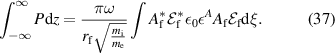
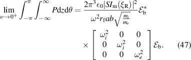
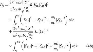
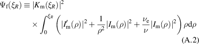
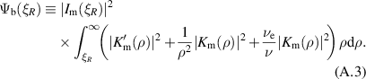
The power loss density P, in SI units, is [22]
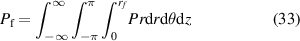
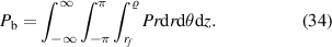
The total power absorbed within  is
is

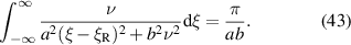
We want to calculate the total power in the  limit
limit

Taking the limit  is a mathematical convenience, in practice the integrands vanish within a few SW decay lengths away from the filament surface.
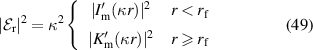
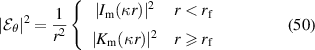
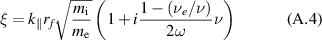
It will be useful to reparametrize (4) and (5) in terms of the dimensionless quantity  . Then
Let us now integrate over z (i.e. along B, along the filament). The length of the filament is much larger than its radius. We approximate the finite filament by taking the integral from  to
to  . In reality, the filaments have finite length, and the ones outside of the last closed flux surface end where they intersect the divertor. See appendix
Integrating also over the azimuthal angle, and inserting (28) (recall  are background quantities, hence the factor R),
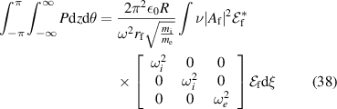
Let the resonance be at  , i.e.
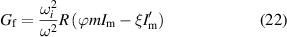
  obeys (25). We linearize the denominator of (20) around the resonance,

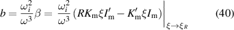
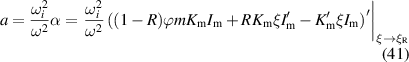
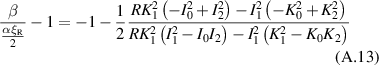
where the prime is the derivative w.r.t ξ at constant R. The dimensionless quantities α and β defined in (40) and (41) are shown in figures 4 and 5. We will soon see that the power P0 scales with  . From these figures, we see that for blob filaments at constant
  , α and β decrease with increasing
  , so the power increases with increasing
  . Thus, resonant interactions not only become rarer at lower
  , they also lose less power.
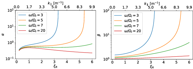
Figure 4. The quantities α and β defined in (40) and (41), which characterize the resonant amplitudes  and
and  as Lorentzians, for blob filaments. We show
  on the upper x axis, with
  assuming deuterium plasma and
  cm.
cm.
Download figure:
Standard image High-resolution image
Figure 5. The quantities α and β defined in (40) and (41), which characterize the resonant amplitudes  and
and  as Lorentzians, for hole filaments. We show
  on the upper x axis, with
  assuming deuterium plasma and
  cm.
cm.
Download figure:
Standard image High-resolution imageAt this point, we note that  behaves, in a neighbourhood of the resonance/pole, like a Lorentzian. As we approach the
  limit,
The factor  becomes higher but more narrowly peaked around
  as ν approaches 0, such that its integral remains finite even in the
  limit. We find this integral by complex contour integration. The poles are at
  , and the corresponding residues,
  , do not depend on ν. Thus
We have the following 'Dirac delta-like' behaviour
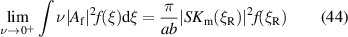
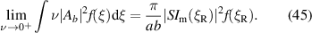
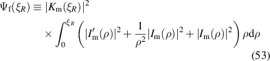
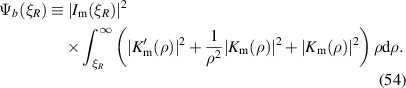
Thus, in the filament
Similarly, in the background
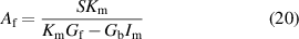
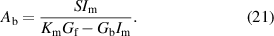
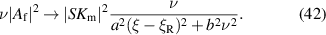
P0, the total power converted to the surface wave mode, is then simply
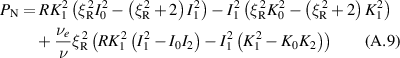
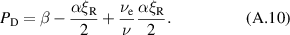
Thus,
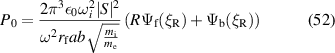
where
Inserting S from (24) and α and β from (40) and (41) into (52):
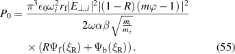
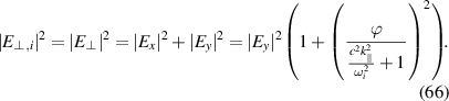
Recall that  is the power spectrum of the perpendicular component of the incident FW electric field, in units of V2. Thus, P0 has units of power. There is also a resonance at
  , and the total power converted by the filament is the sum of P0 over both resonances. If
  is a symmetric power spectrum, this amounts to doubling P0.
4. Filament statistics
Since all the RF calculations in this work are performed within linear electrodynamics, the powers dissipated by two filament modes with different resonant  values are additive. Thus, we can calculate the individual power P0 for isolated filaments and then perform a statistical average
  of the individual powers when
  filaments [11] are present simultaneously in front of the antenna. The most important averaging is over
  , the statistics of which have been studied theoretically by [16, 17], and empirically by [10, 11]. Given some probability density function
  , a corresponding probability distribution over the resonant
  ,
,  , can be readily derived using (25)
Then
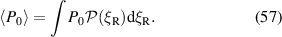
Equation (57) is a bilinear operator from the power spectrum and the probability density to the expected power lost per filament  .
.
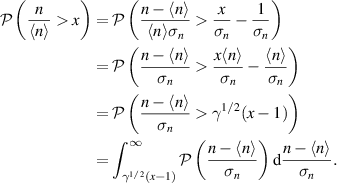
Garcia et al [16, 17] predict that  , where n is the fluctuating density,
  is the time-averaged background density, and σn
is the standard deviation of the fluctuating density, obeys a Gamma distribution
is the time-averaged background density, and σn
is the standard deviation of the fluctuating density, obeys a Gamma distribution
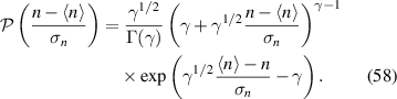
The parameter γ is the so-called 'intermittency parameter'  . From all this, we can derive the cumulative distribution function
Let 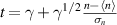 ,
,  ,
, 
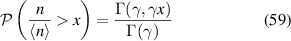
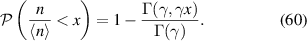
Identifying  with
with  , the probability distribution function is
The probability that a given filament is a blob filament (R > 1) is
The probability that a given filament is a hole filament (R < 1) is
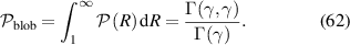
The probability that a given filament interacts resonantly with the incident HHFW (that is, ![$R\not\in[\frac{\varphi-1}{\varphi+1},\frac{\varphi+1}{\varphi-1}]$](https://content.cld.iop.org/journals/0741-3335/64/3/035001/revision2/ppcfac3cfeieqn147.gif) , the band where (25) has no solutions) is
, the band where (25) has no solutions) is
For completeness, we note that very recently, Biswas et al [23] argued that  should be given by a bivariate skew-normal distribution, with a positive correlation between R and
  .
.
5. Example
To show that the power involved in this mechanism is not in general negligible, we consider some NSTX-like values. First, we must assume a power spectrum. Let the spectrum of the vertical component of the incident FW be a simple dipole of amplitude Ai
, peaking at 
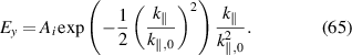
The power spectrum we need is that of the perpendicular component of the incident fast wave. Within the HHFW limit
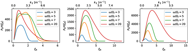
In figure 6, we show  , the curves whose integral gives
  , assuming deuterium plasma with
  m−3,
m−3,  3 m−1,
  –3 cm, and
  V, numbers roughly representative of the NSTX SOL [3, 11]. We see that
  is typically in the order of multiple kW. Considering the presence of tens or hundreds of filaments in the SOL [10, 11] at all times, a considerable fraction of the incident
  MW of power can be lost to surface wave excitation on filaments in NSTX-like conditions. Furthermore, the power lost due to this mechanism is proportional to
  i.e. to the density, and indeed, the HHFW heating in NSTX is more efficient at lower edge densities [24]. Thus, we expect this mechanism to be among the factors responsible for the observed edge losses on that machine [1, 2].
Figure 6.
 , the curves whose integral gives the average power converted to surface wave modes for a blob filament, assuming an incident Ey
spectrum of the form (65) peaking at
, the curves whose integral gives the average power converted to surface wave modes for a blob filament, assuming an incident Ey
spectrum of the form (65) peaking at  m−1 and γ = 2. The filament radius
  is 1 cm (left), 2 cm (middle), and 3 cm (right). The curves with
  integrate to
  kW,
kW,  kW, and
  kW respectively.
Download figure:
Standard image High-resolution image
6. Conclusion
We have discussed a resonant loss mechanism for high harmonic fast waves in tokamak edge plasmas. This loss mechanism is associated with the resonant excitation of surface waves on naturally occurring plasma filaments.
We have derived this loss mechanism for the specific case of resonant surface waves in HHFW-heated plasmas, where the resonant surface wave excitation is approximately described by the result of section 2. The derivation of this loss mechanism does not depend on details of the resonance condition. Analogous loss mechanisms likely exist for any resonantly excited surface wave. If resonant wave–filament interactions occur for heating systems other than HHFW, such as lower hybrid [25], it is likely that similar loss mechanisms are relevant there as well.
Throughout this paper, we interpret P0 as the power lost from the incident fast wave, and transferred to the surface wave along the filament. In this interpretation, it is a transfer of power from one wave mode to another, which is seen as a loss from the point of view of using the incident wave for heating or current drive, but physically the power is not dissipated, it ends up in the other mode. The ultimate fate of this mode-converted power cannot be described by our model (see appendix
Finally, from the estimate we provide for NSTX-like parameters, we find that in a HHFW heating or current drive scenario, this mechanism can easily redirect several kW of power per filament. Further work will focus on the detailed application of this theory to the case of the HHFW edge losses observed in NSTX.
Data availability statement
All data that support the findings of this study are included within the article (and any supplementary files).
Acknowledgments
This work has been carried out within the framework of the EUROfusion Consortium and has received funding from the Euratom research and training programme 2014–2018 and 2019–2020 under Grant Agreement No. 633053. The views and opinions expressed herein do not necessarily reflect those of the European Commission.
J R Myra was supported by the US Department of Energy Office of Science, Office of Fusion Energy Sciences under Award Number DE-AC05-00OR22725/4000158507.
We acknowledge fruitful discussions with Nicola Bertelli and Syun'ichi Shiraiwa of PPPL, and thank Vladimir Bobkov for careful reading and comments.
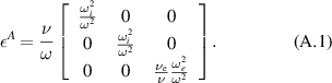
Appendix A.: Independent electron and ion collision frequencies
If we interpret ν as a physical collision frequency, we may want to use a different collision frequency for ions and electrons. Let the ion frequency be ν and the electron frequency  , usually with
  , from momentum conservation considerations
  . Then, we replace (28) by
We take the collisionless limit keeping the ratio  constant. This has two main consequences. First, it changes (54) to
Note that  are now first degree polynomials in
  .
.
Second, it modifies ξ
which affects the linearisation (39)

so a remains as it was in (41), but b gets an extra term, it becomes a first degree polynomial in  . Thus, both the numerator and denominator in P0 (52) are now first degree polynomials in
  . Remarkably, the polynomial in the numerator is proportional to the polynomial in the denominator: the dependence on
  cancels out. P0 (52) does not depend on
  . We prove the case of blob filaments (m = 1). To show that the ratio
  is independent of
  , we need to show that
  . We apply this observation to the numerator polynomial
  , obtained by working out the integrals (A.2) and (A.3)
and the denominator polynomial  which follows from (A.8)
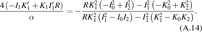
Making use of Bessel function identities, and eliminating ϕ using (26), we can simplify the expression for α to

and the constant term in (A.9) to
The condition for independence of  , the ratio of the constant coefficient over the linear coefficient for the numerator polynomial, must equal that of the denominator polynomial, becomes
Insert (A.11)
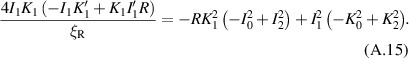
Working out the derivatives on the lhs and  and
and  on the rhs,
which is clearly true.
Appendix B.: Finite filaments
Our model is only valid in a strict sense for infinite magnetic field lines, where the parallel integration (37) can be performed from  to
to  . Yet one would like to use this model for interpreting spurious interactions in the SOL of tokamaks, where open magnetic field lines connect to the material walls. In the presence of dissipation (ν > 0), the nearly-resonant wave-filament modes have a small yet finite spectral width in the
  domain. From the full width at half maximum of the Lorentzian (42)
Our model is an asymptotic theory valid for ν 'small enough', such that  is far smaller than any other spectral scale-length in the problem (this is the condition for the 'Dirac delta-like' relations (44) and (45) to hold). Spatially, the nearly-resonant wave-filament modes should have a large yet finite parallel extent
  . This is the length scale over which the SW fields have non-negligible amplitude, as well as the length scale over which the mode-converted RF power is fully dissipated in the plasma (filament) volume. It is reasonable to think that our approach remains valid for bounded domains if the parallel extent of the nearly-resonant modes is smaller than the typical connection length
  of open magnetic field lines. This leads to the criterion

which defines a lower bound for the parameter ν. It is possible that in a more complete treatment of this problem, a small contribution of the scattered propagative fast wave (which we neglected in this work) will provide a natural lower bound to the losses. If (B.2) does not hold, if  , we expect that not all the estimated mode-converted power can be dissipated in the finite filament in a single pass. Non-negligible RF fields can then reach the field line endpoints. There, they may be partially reflected back to the plasma, partially absorbed by lossy metallic walls, and/or excite sheath oscillations and enhance heat loads to the wall via sheath rectification. However, our model does not capture what happens at these endpoints and is less reliable in assessing the lost power in this regime.