
Abstract
At the ASDEX Upgrade tokamak the electron temperature (Te) profile is estimated from electron cyclotron emission (ECE) using radiation transport forward modeling within the integrated data analysis scheme. For the interpretation of ECE measurements in high  plasmas, it was necessary to upgrade the forward model with a fully relativistic absorption coefficient including the relativistic Maxwell–Jüttner distribution. This model intrinsically enables the interpretation of ECE measurements affected by the so-called 'pseudo radial displacement' or by harmonic overlap. A numerically efficient implementation allows for the analysis of everyday ECE measurements at ASDEX Upgrade. Various ASDEX Upgrade plasma scenarios are discussed highlighting the benefits of the present radiation transport forward modeling for routine analysis.
Export citation and abstract BibTeX RIS

Original content from this work may be used under the terms of the Creative Commons Attribution 3.0 licence. Any further distribution of this work must maintain attribution to the author(s) and the title of the work, journal citation and DOI.
1. Introduction
Electron cyclotron emission (ECE) is one of the primary diagnostics for estimating the electron temperature (Te) profile in magnetically confined fusion research [1].
A calibrated ECE diagnostic measures the radiation temperatures (Trad) for a set of measurement frequencies ω. Often it is possible to infer electron temperature (Te) from Trad via the Rayleigh–Jeans law [2]. The position of the Te measurement is determined by ω and is usually mapped to the cold resonance position, where ω is either equal to the fundamental or an harmonic of the cyclotron frequency [2]. Most frequently the radiometer is optimized such that the second harmonic eXtraordinary mode (X-mode) is the main contributor to the observed Trad.
However, this ubiquitous approach to interpret the ECE measurements becomes inadequate if (I) emission from plasma layers other than the cold resonance position contributes either due to relativistically down-shifted emission or due to Doppler-shifted emission in case of oblique lines of sight (LOS). The same applies if (II) the optical depth of the measurement is low, or if (III) harmonic overlap occurs. For low absorption near the cold resonance, emission from additional plasma layers can pass through the cold resonance layer resulting in a shine-through of down-shifted emission. This occurs typically near the plasma edge and in the near scrape-off layer (SOL) in high-confinement mode (H-mode) plasmas, where emission from the pedestal top and the gradient region is observed in channels with cold resonance positions in the near SOL region. The shine-through radiation causes the Trad profile to show a peak structure in the near SOL, which is called a shine-through peak [3, 4]. Low optical depth at elevated temperatures ( ) can result in shine-through of heavily down-shifted emission from relativistic electrons at the plasma core. Furthermore, even in the case of a large optical depth, a locally small absorption in the plasma core can result in a so-called 'pseudo radial displacement' [5] of the ECE measurements near the plasma core.
To overcome the density cut-off of the second harmonic X-mode, measurements of the third harmonic X-mode spectrum can be used. However, this poses the problem of harmonic overlap, i.e. in addition to the emission from the third harmonic resonance located at the low-field side (LFS), there can be also (at low torus aspect ratio) a contribution by the resonance with the second harmonic located at the high-field side (HFS). Finally, for oblique LOSs the Doppler effect can displace the origin of the observed radiation from the cold resonance position [6, 7].
Radiation transport modeling [4, 7–10] in the framework of Integrated Data Analysis (IDA) [11] allows one to resolve all of these issues. A reliable reconstruction of Te profiles in H-mode from ECE measurements considering shine-through emission and Doppler broadening is obtained for second harmonic X-mode spectra at relatively large electron density (ne) and moderate Te applying a previous electron cyclotron emission forward model (ECFM) [4]. In the present work the radiation transport model presented in [7] is applied, which extends the applicability of the radiation transport method to high Te and ECE measurements affected by third harmonic emission.
This paper is structured as follows. In section 2 the ASDEX Upgrade profile radiometer is presented. In section 3 the radiation transport models described in [7] and [4] are compared. Section 4 shows new applications of the advanced forward model. Conclusions are drawn in section 5.
2. The ECE diagnostic at ASDEX Upgrade
At ASDEX Upgrade a 60-channel heterodyne radiometer is used for ECE measurements. The LOS of the ECE system are close to the mid-plane and the antennae are located at the LFS [4, 12]. Figure 1 illustrates the optics of the ECE diagnostic. A quasi-optical system of three lenses focuses the radiation emitted by the plasma into a rectangularly arranged bundle of waveguides with three rows and four columns. These waveguides are illustrated by the small rectangles on the left side of figure 1. For clarity only the optical paths of two waveguides are shown in each of the figures. The axis of the quasi-optical system, which is shared with an ECE imaging diagnostic [13], is aligned with the center of the wave guide bundle. The waveguides are all parallel to each other and since there are four columns, none of the LOS is perfectly radial. For the two inner waveguides the toroidal viewing angle (i.e. the deviation from a perfectly radial view) is  and for the two outer waveguides
  .
.
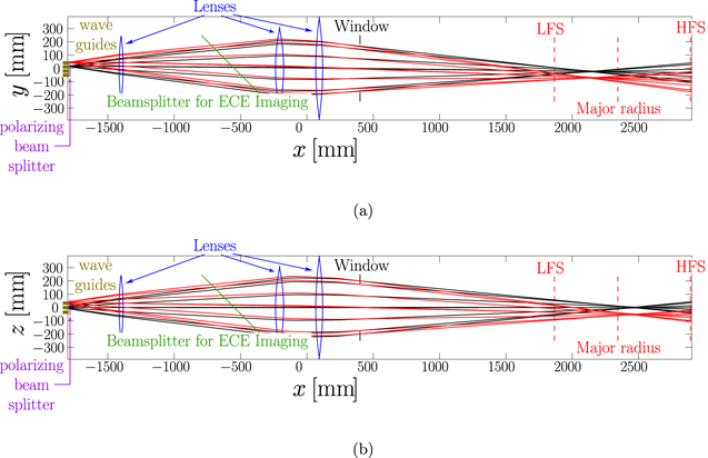
Figure 1. The optics of the ASDEX Upgrade profile radiometer viewed from (a) the top and (b) the side. Black/red lines represent the optical path of the inner/outer waveguides, which are indicated by the brass colored rectangles on the left of the figure. The position of the LFS and HFS wall as well as the major radius of ASDEX Upgrade are indicated by the vertical, dashed red lines on the right side of the figures.
Download figure:
Standard image High-resolution imageThe ASDEX Upgrade profile radiometer is designed to observe the emission of the second harmonic X-mode. In this paper the designation of X and O-mode refers to a propagation perpendicular to the magnetic field. The polarization filter is a wire grid aligned with the toroidal direction of the torus. Because of this alignment the filter is not 100% efficient, due to a small but non-zero pitch angle of the magnetic field and the deviation from a perfectly radial view of the diagnostic. Nevertheless, for this paper it is assumed that the contribution of O-mode radiation to the measurements is negligible. Accordingly all synthetic spectra shown in this paper are pure X-mode spectra. The validity of the assumption of 100% X-mode emission is discussed in section 3.7.
The radiometer covers a frequency range from 84.3 to 143.6 GHz. For ASDEX Upgrade's typical magnetic field strength ( 2.5 T) the resonance positions are chosen such that they cover a region ranging from a few centimeters on the HFS close to the magnetic axis across the entire LFS and to the SOL. Thirty-six of the sixty channels feature a bandwidth of 300 MHz, which corresponds to a spatial resolution (disregarding frequency broadening effects) of
  at the plasma edge. The channels are distributed non-equidistantly with a typical spacing of 400 MHz. The other 24 channels have a wider bandwidth of 600 MHz and a frequency spacing of approximately 1 GHz. This translates into a spatial resolution of
  at the plasma core. The profile radiometer is absolutely calibrated with the hot–cold source technique [14]. The estimated systematic error of the calibration is 7%. The ECE measurements are sampled with a frequency of 1 MHz. The measurements shown in this work are averaged over 1 ms. The error bars are evaluated from the sum of squares of the systematic uncertainty and one standard deviation from the temporal average.
3. The improved radiation transport model
The previous ECFM [4] is compared with the present, improved radiation transport model [7] by using plasma scenarios with significant shine-through from the core to the edge due to heavily down-shifted emission of relativistic electrons. However, a straightforward comparison of the ECFM presented in [4] with the improved radiation transport model proposed in [7] is not possible. For the selected scenarios the model of [4] faces issues with numerical stability and validity limitations. It is emphasized that these problems arise only for the type of scenarios addressed in this paper, whereas the results presented in [4] are not affected. Three modification are made to the previous ECFM [4] for the benchmark against the improved radiation transport model of [7]:
- 1.In the model from [4] the cut-off density of the second harmonic X-mode was approximated with
 , with
  0 the vacuum permittivity, the cyclotron frequency, B the total magnetic field strength, me,0 the rest mass of the electron and e the elementary charge. This approximation assumes that the measurement frequency ω equals twice the cyclotron frequency. While this approximation holds at the cold resonance position of the second harmonic, it is invalid for strongly down-shifted emission for which ω < 2ωc,0. Instead, the cold plasma refractive index is used to identify the regions of the LOS where the microwaves are evanescent. This is also consistent with the cold plasma raytracing performed in the improved radiation transport model of [7].
 - 2.The analytical solution of the emissivity integral presented in [4] is observed to be numerically unstable for strongly down-shifted emission ω < 2ωc,0. The stability issues are caused by the numerical implementation of the Dawson Integral which is required by the analytical formula. Replacing the analytical solution of the integral with a Gaussian quadrature scheme avoids this issue.
- 3.The forward Euler solver for the radiation transport differential equation is replaced with a 4th order Runge–Kutta integrator, which improves numerical stability.


From this point on the ECFM of [4] including the modifications explained above is denoted as model A. The model presented in [7] will be referred to as model B.
3.1. Similarities between the two models
Both models, A and B, first calculate the LOS and then solve the radiation transport equation along the LOS in a second step. Both models assume a thermal plasma and apply Kirchhoff's law relating the emissivity and the absorption coefficient. For the comparison only the second harmonic X-mode emission is considered, because unlike model B, model A was not designed for any other harmonic or wave polarization. Furthermore, an infinite reflection model is used in both models to include the effect of wall reflections [4, 7, 15]. The wall reflection coefficient is chosen to be Rwall = 0.9 for all calculated Trad profiles in this paper. This value has been proven to be reasonable for most ASDEX Upgrade plasmas that exhibit a shine-through peak.
3.2. Improvements
For a general treatment of electron cyclotron waves the relativistic dispersion relation has to be solved for the complex refractive index  [16]. Unfortunately, no analytical solution is available and numerical schemes [16] become unreliable if roots corresponding to electrostatic Bernstein waves [17] lie close to or coincide with the roots of the X- or O-mode [18].
A compromise between the general treatment and the approximations used in [4] is provided for model B by combining the absorption coefficient given by equation (7) of [19] with cold plasma geometrical optics raytracing. Cold plasma geometrical optics raytracing for ECE is a standard procedure [8, 10], but, to our knowledge, the application of the absorption coefficient of [19] is new.
The approach of [19] inherently considers only the electromagnetic energy flux while the so-called sloshing flux, which is non-zero only if finite temperature effects are included in the dispersion relation, is neglected [19, 20]. Furthermore, the refractive index Nω and the wave polarization vector are derived from the cold dielectric tensor. The advantage is that the absorption coefficient and the emissivity are expressed as an integral in momentum space that can easily and robustly be solved numerically. The details on the absorption coefficient and the emissivity can be found in appendix A. With these approximations the emissivity and absorption coefficient of model B are typically about 10% different from the values derived rigorously from the fully relativistic dispersion relation. Nevertheless, as shown in appendix B, the modeled ECE intensities do not differ significantly as long as the optical depth is not too small.
With the modified emissivity, absorption coefficient and the addition of geometrical optics raytracing, the four key improvements of model B relative to model A are:
- 1.
- 2.
- 3.
- 4.
3.3. Significance of improvements
In order to assess the significance of the various improvements implemented in model B, a hybrid model  is introduced containing all improvements (1–3) except for the relativistic distribution function (4).
Figure 2 compares the radiation temperature Trad evaluated with models A,  and B (Trad,mod) with the measured values Trad,ECE for three different scenarios. All three scenarios have strong, central electron cyclotron resonance heating (ECRH), a correspondingly large Te in the plasma core, and an on-axis magnetic field strength of about
  . The main distinction is given by different on-axis electron densities ne: (a) #31594 at
  has a very low plasma core density of
  (b) #32740 at
  is in mainly helium with a plasma core density of
  (c) #31539 at
  has a comparatively large plasma core density of
  . The ne values are summarized in table 1.
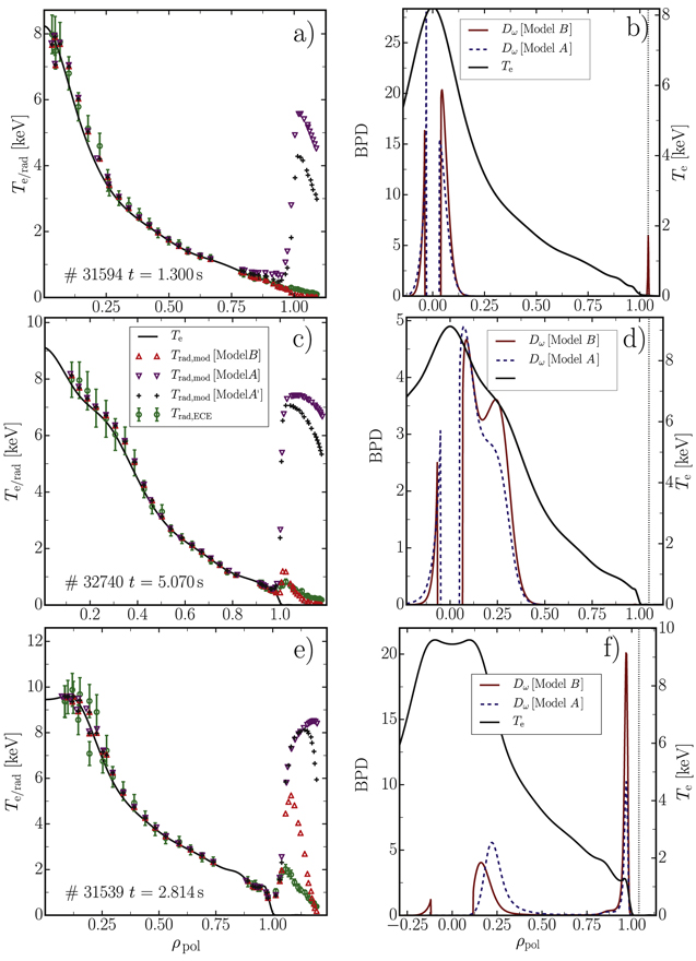
Figure 2. (a), (c) and (e): Estimated Te profiles applying radiation transport modeling in the IDA scheme as functions of  . Additionally, the modeled Trad,mod according to model A,
  and B are compared to the measured Trad,ECE. Both, synthetic and actual measurements are mapped to the cold resonance position of the second harmonic. (b), (d) and (f) illustrate the birthplace distributions of observed intensity, as calculated by the models A and B, for a channel with a cold resonance position of
  (dotted vertical line) for the three plasma scenarios of (a), (c) and (e).
Download figure:
Standard image High-resolution imageTable 1. The core electron density values of the three benchmark scenarios.
| Shotnumber | ne |
|---|---|
#31594, 
|
|
#32740 
|
|
#31539 
|

|
The Te profiles shown in figures 2(a), (c) and (e) are functions of the square root of the normalized poloidal flux, ρpol. The Te- and ne profiles are estimated within the IDA framework combining measurements from ECE, interferometry [21] and lithium beam spectroscopy [22] for #31594 and #31539. Thomson scattering [23] measurements of ne replace the lithium beam spectroscopy measurement for #32740, because overlapping lithium and helium lines reduce the reliability of lithium beam spectroscopy in helium plasmas. The ECE measurements in figures 2(a), (c) and (e) are mapped to cold resonance positions. The Te profile is inferred from the ECE measurements with model B. Only ECE measurements within the confined region (ρpol < 1) were considered. Therefore, the comparison of the measured and forward modeled Trad in the SOL ( ) allows one to validate the various models.
For channels with cold resonance positions in the SOL, model B provides the best agreement between the measured and modeled Trad even though these channels are not considered in the fit. Model A shows the worst agreement. Model  including three out of the four improvements performs only little better compared to A. Although model B describes the relatively small measured ECE intensities at the outer edge reasonably well, there are residual discrepancies, especially in #31539 (see figure 2(e)). The residual discrepancy is discussed in sections 3.5 and 3.6.
In most plasmas there is no significant difference between the Trad of models A and B inside the confined region (see figures 2(c) and (e)). However, model A performs poorly if Te and ne are extremely small in the edge of the confined region (see figure 2(a)). Such conditions arise at ASDEX Upgrade routinely in ohmic discharges which necessitates the analysis with the extended model B.
3.4. Relativistic versus non-relativistic distribution function
For the scenarios studied in [4] with relatively large ne ( ) and moderate Te (
 ) the measurements and forward modeled Trad were consistent. This was confirmed with model B. The different performances of models A,
  and B for the present plasma scenarios mainly results from the different electron energy distribution functions considered and the shine-through of down-shifted emission from relativistic electrons in the plasma core. The origin of the radiation is given by the birthplace distribution of observed intensity (BPD) [6, 7]. The BPD of ECE measurements corresponds to the power deposition profile of the ECRH being normalized to the total deposited power, whereas the BPD is normalized to one. Figures 2(b), (d) and (f) compare the BPDs from models A and B for the cases of figures 2(a), (c) and (e), respectively. Negative (positive) values of ρpol correspond to positions on the HFS (LFS), respectively. The gap in the BPDs close to the plasma center arise from the LOS not going exactly through the plasma center. The ECE channel was chosen such that its cold resonance position lies at ρpol ≈ 1.04 (dotted line).
All three cases show a significant contribution of the plasma core which decreases with increasing density as is expected due to the increased optical depth. This contribution was not observed for the scenarios discussed in [4]. The large SOL peaks in Trad predicted by models A and  result from an overestimation of the strongly down-shifted radiation from electrons in the tail of the electron velocity distribution located in the plasma core. The Maxwell distribution does not account for the relativistic mass increase resulting in an over-population of the relativistic speeds. The contribution of down-shifted emission to ECE measurements is known since long [3, 24, 25], but associated with non-thermal electron velocity distributions. Studies of non-thermal distribution functions analyzing ECE data use, e.g., a non-relativistic Bi-Maxwellian [25–27]. However, strongly down-shifted ECE arises already from the thermal tail of the distribution function. With an on-axis magnetic field strength of
  the second harmonic of the cyclotron frequency is
  in the plasma core. In contrast, the measurement frequency fECE of the channels for which the cold resonance positions lie in the SOL is only about 105 GHz. If the down-shift is attributed to the relativistic mass increase alone (i.e. if the Doppler shift is neglected), a Lorentz factor of γ = 1.4 is required. This corresponds to an electron velocity
  , where c0 is the vacuum speed of light, and a kinetic energy of about
  . Figure 3 compares the Maxwellian with the Maxwell–Jüttner distribution for
  . For
. For  the Maxwellian is significantly larger than its relativistic counterpart. The position on the LOS contributing the most to the observed, strongly down-shifted emission is given by the local maxima closest to the magnetic axis of the BPDs shown in figures 2(b), (d) and (f). For each point on the LOS it is possible to derive the velocity β which contributes strongest to the observed down-shifted emission using the resonance condition and the integrand of the emissivity. With the BPD the position that has the strongest contribution of down-shifted emission can be identified. By combining these two pieces of information the velocity that contributes the most to the down-shifted emission can be calculated. This velocity is indicated by the vertical lines in figure 3. The variability of β from 0.55 to 0.60 is due to different Doppler shifts and BPDs. The scenario with the smallest (largest) ne shows the region with largest (smallest) frequency down-shift.

Figure 3. Maxwellian and Maxwell–Jüttner distribution for Te = 8 keV. The velocities with the largest amount of down-shifted emission for the SOL channels shown in figures 2(b), (d) and (f)
Download figure:
Standard image High-resolution image3.5. The Abraham–Lorentz force
Model B describes small Trad values in the SOL region reasonably well for plasmas with either low Te or low ne, e.g., for the discharges #31594 and #32740. But it overestimates Trad for plasmas with large core Te and  , e.g., for #31539. Reference [28] shows that the radiation drag can reduce the efficiency of electron cyclotron current drive in future fusion devices by depleting the high-energy tail of a thermal distribution. Therefore, the omission of the Abraham–Lorentz force [29] is investigated as a possible reason for an overestimation of Trad. Although the radiation drag was found to be negligible for the presented ECE measurements, the approach is described to allow for further evaluation of ECE measurements in future plasma scenarios.
For estimating the effect of the Abraham–Lorentz force on ECE measurements the radiation drag has to be balanced with thermalizing collisions. For small velocities the radiation reaction force is expected to be negligible as the collision frequency is large. For relativistic velocities the radiation reaction force is expected to alter the thermal distribution due to a relatively small collision balancing term. To estimate the significance of the radiation reaction force on ECE measurements the linear solution for the steady-state electron distribution function resulting from the Abraham–Lorentz force [30, 31] and relativistic collisions [32] was calculated analytically assuming a homogeneous plasma and a dimensionless momentum  . The details on the calculation can be found in appendix C. The steady-state distribution
Taking into account the radiation reaction force, is expressed as a sum of Legendre polynomials Pn with the pitch angle  as argument. The pitch angle is given by the fraction of u∥ the dimensionless momentum parallel to the magnetic field over the dimensionless, total momentum u. The coefficients of the Legendre polynomials gn are given by:
It can be shown that all other coefficients (g1, gn > 2) are zero. The following variables were introduced in equations (2) and (3):
where Z the effective charge and  the Coulomb logarithm. For the calculations the mean value of B on the flux surface and Z = 1.5 is considered. Note that the distribution function given by equation (1) has to be multiplied by a factor to ensure normalization. However, the normalization factor differs only very slightly from one, because only f0g0, which is of the order of 1.0 × 10⁻⁵, contributes to the normalization.
This analytical solution was compared with the numerical solution obtained with the Fokker–Planck code RELAX [33], which was extended to include the Abraham–Lorentz force. The deviation of the two non-thermal distributions from the thermal distribution was computed and normalized by the value of the thermal distribution. These normalized deviations are shown in figure 4(a) as functions of the dimensionless momentum perpendicular to the magnetic field  for u∥ = 0 and ρpol = 0.2. Both distributions show a depletion of high-energetic electrons of the order of 5%–20% in the relevant range of u⊥ = 0.6–0.8.
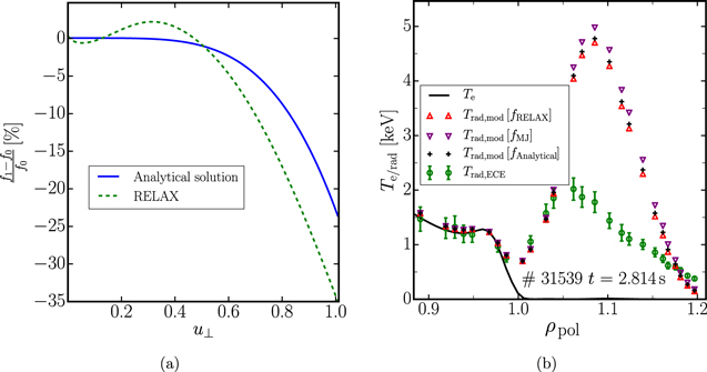
Figure 4. (a) The normalized deviations from a thermal distribution due to the Abraham–Lorentz force are shown for the analytical solution and the distribution function calculated by RELAX for ζ = 0. (b) Comparison of the forward modeled Trad considering the analytically computed distribution, the distribution function from RELAX, and a thermal distribution.
Download figure:
Standard image High-resolution imageThe expressions for the emissivity and the absorption coefficient given in appendix A allow Trad to be computed with model B even in case of non-thermal distributions. In figure 4(b) Trad derived from the analytical distribution function profile and the distribution function profile of RELAX are compared to the thermal Trad profile for the ECE channels with resonance positions in the SOL. The reduction of Trad compared to the Trad evaluated with a thermal distribution function is only in the order of a few %. This clearly shows that the effect of the Abraham–Lorentz force is too small to be responsible for the overestimation of Trad. The observed discrepancy between the modeled and the measured Trad must therefore have a different reason.
3.6. Wall reflections
Another possible reason for the overestimation of Trad is given by the simplicity of the infinite wall reflection model. Figure 5 compares Trad,mod computed with the wall reflection coefficients Rwall = 0.9 and Rwall = 0 (no reflection). The much better agreement of the measurements with the modeling without wall reflections indicates that for this discharge wall reflection might be overestimated.
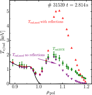
Figure 5. The forward modeled Trad with and without wall reflections are compared to the ECE measurements in the SOL of discharge #31539.
Download figure:
Standard image High-resolution imageThis appears to be plausible since the infinite wall reflection model is known to be inappropriate if the optical depth is very small [15]. In #31539 the optical depth of the plasma for channels with resonance position ρpol,res > 1.04 is τω < 0.2. For this situation and assuming an idealized case of a perfectly reflecting wall (Rwall = 1) more than 15 direct reflections are needed to provide a total optical depth τω > 3. For these cases, it is expected that the entire plasma volume contributes to the ECE measurement [34]. Reference [15] suggests to assume that the radiation from the plasma is in thermal equilibrium with the wall. The wall then provides an initial radiation temperature to the radiation transport equation resulting in a significantly smaller intensity at the ECE antenna compared to the infinite wall reflection model. However, the formalism of [15] is not directly usable for radiation transport modeling, since it is assumes that only emission from cold resonance positions contributes to the measurements. This is clearly not valid for the SOL ECE channels of, e.g., scenario #31539 (see figure 2(f)), where there is no significant contribution from the cold resonance position. For ECE measurements in the mid-plane it is expected that a generalized form of the reflection model of [15] results in a significantly smaller enhancement of Trad than the infinite reflection model predicts. A detailed comparison between the infinite wall reflection model and an appropriately extended version of the reflection model of [15] will be subject of future work.
To conclude, for optical depths below about τω < 0.5 the infinite reflection model does not provide reasonable values for Trad. Additionally, for low density, primarily electron heated plasmas (e.g. #31594 and #32740) the situation complicates, because the ECRH might give rise to non-thermal distribution functions. Fast electrons are known to be able to affect the ECE measurements of the SOL significantly [35]. In #31539 a significant influence of fast electrons is not expected due to the relatively large core density.
3.7. O-mode
Due to the toroidal alignment of the polarizing beam splitter a small fraction of the X-mode ECE is reflected and a corresponding fraction of O-mode emission can pass through. In routine analysis it is assumed that only X-mode emission contributes but with 100% of its intensity. The X-mode Trad is typically much larger than the O-mode Trad because of the rather low optical depth of the second harmonic O-mode ECE in ASDEX Upgrade plasmas. Hence, assuming 100% X-mode erroneously results in an overestimation of Trad. To investigate the relevance of this overestimation, the radiation transport model presented in [7] was extended to include the polarization filter:

Hence, the synthetic radiation temperature becomes a sum of the O-/X-mode radiation temperature  which is weighted by the transmissivity of the polarizer. The transmissivities of the polarizer for each mode is computed by projecting the normalized polarization vector of the O-/X-mode
  onto the polarization axis of the filter
  .
.
The modeling of the polarization filter shows that 5%–10% of the O-mode ECE can pass through the filter. The fraction depends on the toroidal angle of the antenna and the ratio between the poloidal and the toroidal magnetic field strength in the mid-plane. Correspondingly, the X-mode contribution is reduced by the same fraction. Wall reflections are expected to mitigate the rather small optical depth of the O-mode emission (τω < 0.2). Assuming the infinite reflection model the calculated Trad spectra superposed by the O- and X-mode are at most 5% smaller than the pure X-mode spectra. Neglecting reflection completely, results in Trad of the combined O- and X-mode spectrum being 5%–10% smaller than the pure X-mode spectrum.
Although 5%–10% overestimation of Trad might be significant in special applications, for routine analysis it is considered to be negligible. The code allows one to optionally include (switch on) the filter effect and the O-mode contribution but at the cost of increased numerical effort.
4. Applications of electron cyclotron radiation transport modeling
In standard plasma scenarios with relatively large ne and moderate Te, radiation transport modeling describes the shine-through peak at the plasma edge as down-shifted emission from the pedestal top through the steep H-mode pedestal gradient without the need for non-thermal electrons [4]. For routine evaluation of ECE measurements in a broad operational space, radiation transport modeling has to reliably describe the effects observed in all plasma scenarios. This includes the two cases: 'pseudo radial displacement' in the plasma core and measurements affected by harmonic overlap.
4.1. 'Pseudo radial displacement' in the plasma core
At high Te and low ne ECE measurements are known to show a 'pseudo radial displacement' [5], which was observed, e.g., at ASDEX Upgrade [36, 37], JET [38], DIII-D [39] and TORE-SUPRA [40]. The 'pseudo radial displacement' is observed for large Te gradients in the plasma core for discharges with large Te and small ne. It results from reduced absorption close to the cold resonance position and a corresponding shining of down-shifted emission through the cold resonance. The 'pseudo radial displacement' is already intrinsically included in the radiation transport model of [4]. However, 'pseudo radial displacement' is observed at ASDEX Upgrade only in high Te discharges where the usage of a non-relativistic Maxwellian is inappropriate for the interpretation of the plasma edge ECE measurements. The improved model allows the consistent description of ECE measurements in scenarios with 'pseudo radial displacement'.
The 'pseudo radial displacement' can best be seen if the ECE channels are mapped to magnetic coordinates, where a loop structure in Trad appears even though Te is expected to be constant on flux surfaces. A similar loop structure might also occur (and is observed) when the flux surfaces of the magnetic equilibrium are inaccurately estimated. The two possible sources of the loop in Trad,ECE(ρpol) can be distinguished by radiation transport modeling. The loop structure by 'pseudo radial displacement' can be described by radiation transport modeling whereas a residual loop not modeled properly with radiation transport could be explained by an erroneous equilibrium. This residual loop structure provides valuable information to improve the equilibrium reconstruction employing iso-flux constraints [41].
Figure 6 shows ECE measurements from discharge #30907 at  with a large Te gradient and a relatively small electron density of
  in the plasma core. Negative (positive) values of ρpol correspond to cold resonance positions on the HFS (LFS), respectively. Trad on the HFS (LFS) is smaller (larger) than Te at the cold resonance position. This displacement is due to the low absorption at the cold resonance position and the shine of down-shifted radiation through the cold resonance [37]. The corresponding modeled Trad,mod values describe the measurements Trad,ECE reasonably well. This indicates that for the present case the equilibrium is not responsible for the displacement. In the chosen scenario the 'pseudo radial displacement' is large compared to the uncertainty of the equilibrium. The equilibrium was validated using tomographic reconstruction of the soft x-ray measurements [42]. For this case the soft x-ray reconstruction allows one to determine the magnetic axis with an upper uncertainty margin of 1 cm. Shifting the magnetic axis by 1 cm in any direction affects the HFS–LFS asymmetry of the ECE measurements negligibly. Radiation transport modeling allows the reconstruction of Te without the need for extra displacement of the emission location as proposed e.g. by [43]. This is very convenient for routine analysis of large data sets.

Figure 6. Loop structure of measured Trad,ECE as a function of the magnetic coordinate and the Te profile estimated using radiation transport modeling in the framework of IDA. In the right figure cold resonance positions on the HFS have negative normalized coordinates.
Download figure:
Standard image High-resolution image4.2. Third harmonic and harmonic overlap
The application of ECE for high ne operation is limited by cut-offs, which is expected to hamper the use of the ECE diagnostic in future fusion devices. One solution to this problem is to measure the emission of a higher harmonic. In the case of ASDEX Upgrade one can measure third harmonic X-mode instead of the second harmonic, which increases the cut-off density by a factor of 1.5 compared to the X2-mode. However, this approach is of limited applicability for two reasons. The first is that the X3 absorption coefficient in medium size devices like ASDEX Upgrade is small. This broadens the BPD significantly compared to the BPD of the second harmonic emission. The second challenge is given by the harmonic overlap. Typically, the cold resonance position of third harmonic ECE lies on the LFS and it can be accompanied by an additional resonance with the second harmonic on the HFS. The combination of the low optical depth of the third harmonic resonance with the harmonic overlap can cause the second harmonic emission from the HFS to shine through the absorption layer of the third harmonic [44]. Hence, in order to estimate the Te profile the mixture of X2 and X3 emission needs to be modeled properly.
An example of harmonic overlap is illustrated in figure 7 for the ASDEX Upgrade discharge #32934 at t = 3.298 s with a magnetic field of  and a plasma core density of
  . Figure 7 shows the corresponding plasma frequency fp, the right-hand cut-off frequency fR, and the fundamental, second and third harmonic of the cyclotron frequency fc. For a measurement frequency of
  the emission of the X2-mode is inaccessible for the entire LFS (R > 1.65 m), because the right-hand cut-off frequency fR > 2fc (see figure 7). In contrast, an increased measurement frequency of
  is not in cut-off, but introduces the problem of harmonic overlap.

Figure 7. #32934 at t = 3.298 s: radial dependence of the first, second and third harmonic of the cyclotron frequency fc, the plasma frequency fp, the right hand cut-off frequency fR and a measurement frequency of 129 GHz.
Download figure:
Standard image High-resolution imageAt DIII-D the harmonic overlap has been addressed by calculating the optical depth of the X3-resonance and by evaluating Trad from the mixture of X2 and X3 radiation under the assumption of Trad = Te at the positions of both cold resonances [44]. Compared to the rigorous treatment employing radiation transport modeling, the DIII-D approach has two disadvantages. The first is that the method of [44] inherently requires Thomson scattering measurements to determine Te at the cold resonance position of the second harmonic. The second disadvantage is that any relativistic broadening of either resonance is neglected.
The radiation transport model in the IDA framework allows one to determine the Te profile by only considering Te information from ECE measurements. This works for any plasma region provided that significant local Te information is supplied by the ECE measurements. Figure 8 shows discharge #32934 at t= 3.298 s where harmonic overlap has to be considered for nearly all channels. In contrast to the previous figures, the measured Trad,ECE are mapped to the cold resonance position of the third harmonic. The black line depicts the Te profile estimated from ECE measurements only. The black dashed lines indicate the upper and lower error band of the Te profile. Although  is matched very well for all measurements, Te is only reliable in the region of ρpol < 0.8. The Te profile has large upper and lower uncertainties for ρpol > 0.8, because the ECE measurements do not provide significant information on the Te profile in this region. Figure 9 shows the BPDs for three selected channels. The black line corresponds to a channel with X2-resonance at
  on the HFS and with X3-resonance at ρpol = 0.48 on the LFS. Only the X3-mode contributes significantly to the measured intensity. The X3-mode emission is broad with a significant contribution of down-shifted ECE. The red line corresponds to a channel with X2-resonance at
  on the HFS and with X3-resonance at ρpol = 0.90 on the LFS. Both harmonics contribute to the measured intensity. The cyan line corresponds to a channel with X2-resonance at
  on the HFS and with X3-resonance in the SOL (ρpol = 1.01). Although mapped in figure 8 to the third harmonic resonance position only X2-mode emission contributes to this channel. The combination of a decreasing contribution from the X3-mode in the LFS region
  and the small X2-mode emission on the HFS for
  results in missing information about Te in this region.

Figure 8. Te profiles and their corresponding uncertainties (dashed lines) estimated from ECE measurements (Trad,ECE) only (Te[ECE]) and from the combined analysis of ECE and Thomson scattering data (Te,TS) (Te[ECE + TS]). The ECE measurements are mapped to the third harmonic cold resonance positions. Both sets of modeled ECE measurements Trad,mod[ECE] and Trad,mod[ECE + TS] agree reasonably well indicating the lack of information in the ECE data for ρpol > 0.8.
Download figure:
Standard image High-resolution image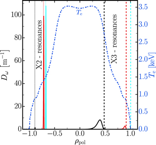
Figure 9. Te profile and the birthplace distributions for three channels shown in figure 8 at 3rd harmonic cold resonance ρpol values of 0.48 (black), 0.90 (red) and 1.01 (cyan). The vertical lines show the 2nd (dotted) and 3rd harmonic cold resonance positions (dashed).
Download figure:
Standard image High-resolution imageAlthough the method intrinsically works without additional diagnostics, improved results in regions with poor ECE coverage can be obtained if the ECE measurements are supplemented with Thomson scattering data. The red line in figure 8 depicts the Te profile of the combined analysis Te[ECE + TS] and the red dashed line the corresponding upper and lower error margins. For ρpol < 0.8 Thomson scattering does not provide significant additional information. It only confirms the ECE measurements. For ρpol > 0.8 the lack of information from ECE is compensated by Thomson scattering. The modeled values Trad,mod[ECE] and Trad,mod[ECE + TS] agree very much indicating that the large error bars for ρpol > 0.8 in the Te profile considering ECE only is indeed resulting from missing information.
5. Conclusions
An improved radiation transport model for ECE is compared to a previous model used for standard plasma scenarios at ASDEX Upgrade. Only the improved model is capable of describing the ECE measurements in the plasma edge and SOL region correctly for plasmas with a core  . The benefits of the extended validity of the new model were highlighted for two plasma scenarios. The improved model extends the pool of plasma scenarios that can be evaluated reliably within the routine analysis.
The improved model includes cold plasma geometrical optics raytracing and a fully relativistic absorption coefficient considering cold plasma dispersion for wave polarization and refractive index. The relativistic Maxwell–Jüttner distribution is the most important new ingredient for describing properly the shine-through of heavily down-shifted emission from relativistic electrons in the plasma core. In addition, the effect of the radiation reaction force on the high-energy tail of the electron distribution function and its consequence for the ECE measurement was investigated analytically and numerically. No significant effect on the modeled Trad was found for the scenarios discussed. The influence of wall reflections was identified as a plausible explanation for the residual discrepancy which remains between measured and modeled Trad for measurements with extremely low optical depth. The radiation transport model of [7] was extended to include the polarization filter, which allowed the estimation of the influence of O-mode emission on the ECE measurements at ASDEX Upgrade. Assuming that purely X-mode emission contributes to the ECE spectra overestimates the modeled Trad by 5%–10% at ASDEX Upgrade.
The improved radiation transport model is applied to two plasma scenarios which constitute special cases from the perspective of ECE. The 'pseudo radial displacement' observed for large core Te gradients is correctly accounted for by the model. The successful reconstruction of Te profiles from ECE measurements containing a mixture of X2 and X3 emission is demonstrated. Supplementing the ECE data with Thomson scattering data in the IDA framework helps to recover regions which are not covered properly by the ECE data alone.
In summary, the IDA approach including the advanced radiation transport forward model considerably improves the accuracy of Te profile reconstructions and extends the operational space of the ECE diagnostic. The ECE forward model is applicable for routine analysis in everyday ECE data interpretation.
Acknowledgments
One of the authors (S S Denk) acknowledges Daniela Farina and Lorenzo Figini, who provided the numerical implementation of the absorption coefficient rigorously derived from the warm dispersion relation [16].
The computations have been performed in part on the EUROfusion Gateway Cluster, using the framework developed and maintained by the EUROfusion-IM Team6 . This work has been carried out within the framework of the EUROfusion Consortium and has received funding from the Euratom research and training programme 2014–2018 under grant agreement No 633053. The views and opinions expressed herein do not necessarily reflect those of the European Commission.
Appendix A.: The absorption coefficient and the emissivity of model B
In this appendix we give a concise account of the expressions of absorption and emission coefficients used in model B. The absorption coefficient provided by [19] is
A similar expression for the emissivity can be derived from equation (2.9) of Bellotti et al [45]. The exact details of the derivation will given in a separate paper on the modeling and computational aspects of this work. The final expression is
where Nr is the ray refractive index,  the plasma frequency and
  is the wave electric field normalized with the absolute value
  of the wave-energy flux vector
  .
.
The Lorentz factor is denoted as  and u∥ and u⊥ are the components of the dimensionless momentum
  parallel and perpendicular to the equilibrium magnetic field, respectively. The momentum distribution function
  can be arbitrarily chosen but the implementation of model B is limited to gyrotropic distributions. The Dirac's δ-function accounts for the cyclotron resonance, with n the harmonic number. At last [19]
where Jn is the Bessel function of first kind with argument  . The components of the refractive index Nω perpendicular/parallel to the ambient magnetic field are denoted as N⊥/∥. If the distribution function f is chosen to be the Maxwell–Jüttner distribution it is possible to reproduce Kirchhoff's law with expressions given by equations (A1) and (A2).
The integrals in equations (A1) and (A2) can be solved numerically if the cold dielectric tensor is considered in the derivation of the refractive index Nω and the normalized polarization vector  as described in [19].
Appendix B.: Validation of the absorption coefficient
For the approximated absorption coefficient given by equation (A1) the refractive index, the polarization vector and the energy flux are derived from the cold plasma dispersion relation. This approximation is valid for any harmonic n > 2 and for the second harmonic (n = 2) if [17, 20]:

But for, e.g.,  which is typical for ASDEX Upgrade, ωc,0 ≈ ωp,0 for
  . For routine data analysis at ASDEX Upgrade the radiation transport model has to perform reasonably well for densities up to the cut-off density
  . Nevertheless, for the analysis of ASDEX Upgrade ECE measurements the approximated absorption coefficient is a viable approximation even if the condition given by equation (B1) is violated. The approximated absorption coefficient is benchmarked against the absorption coefficient derived self-consistently from the solution of the fully relativistic (or warm) plasma dispersion relation (see [16]).
The two absorption coefficients are compared in figure B1(a) for three densities ne =  , ne =
  and ne =
  and a measurement frequency
  . In figure B1(b)
  is chosen and, to avoid cut-off, lower densities ne =
  , ne =
  and ne =
  are selected. In both cases the angle between the magnetic field lines and the wave vector is 85° and Te is 8 keV. For the selected frequencies, all densities and almost for the entire range of
  , there are deviations in the order of 5%–15%. Larger deviations occur for
  in case of the largest ne respectively in figures B1(a) and (b). In contrast to the absorption coefficient from the warm plasma dispersion relation the approximated absorption coefficient does not allow for wave propagation for small
  and large ne.

Figure B1. The approximated absorption coefficient of equation (A1) (sold lines) and the absorption coefficient derived from the warm dispersion relation (dashed lines) are shown for six different ne and two different measurement frequencies fECE = 140 GHz (a) and fECE = 105 GHz (b) as a function of the cyclotron frequency normalized by the measurement frequency.
Download figure:
Standard image High-resolution imageFigure B1 shows, as expected, that the cold plasma dispersion produces the largest errors close to cut-off. Although the relative deviations are in the order of ten percent in the full range of  and all considered ne and frequency combinations, in practical applications, the cold plasma dispersion for the absorption coefficient is sufficient to provide good estimates for Trad for the ASDEX Upgrade ECE diagnostic. To exemplify this, discharge #33596
  is selected for the benchmark of Trad. The peak Te is about 11 keV and ne is about
  , which is similar to the parameters of the benchmark of the absorption coefficients. The magnetic field of the discharge is on-axis −2.5 T and the for data analysis useful channels of the ECE diagnostic cover a frequency range from 110 to 143 GHz. The result of the benchmark of Trad is shown in figure B2. The Te profile used for the benchmark and shown in figure B2 was inferred from the ECE measurements with model B. The ECE measurements and the forward modeled Trad computed with each of the two absorption coefficients correspond to the left y-axis. The right y-axis shows the relative deviation between the two forward modeled Trad. The measurements shown in the red shaded region have optical depths below τω < 0.5 and are not considered in the analysis. Measurements with optical depth τω < 0.1 were removed from the figure. The relative deviations between the two calculated Trad profiles are below 5% for all measurements that enter the data analysis. Only channels with extremely low optical depth τω < 0.5 show a significant deviation between the two forward modeled Trad profiles. For these channels, however, the high sensitivity on the empirical wall reflection coefficient renders the Te information stored in the measurement irrecoverable by the IDA method regardless of which absorption coefficient is used.
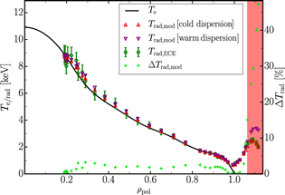
Figure B2. #33596 at  : comparison of Trad calculated with the approximate absorption coefficient and the absorption coefficient derived from the warm dispersion relation. Significant deviations between the two calculated Trad,mod (>5%) occur only for the channels that are highly sensitive to the wall reflection coefficient (red shaded area).
Download figure:
Standard image High-resolution imageAppendix C.: Synchrotron radiation steady-state distribution
We want to find the steady-state distribution function of electrons taking the radiation reaction force into account. In the kinetic equation

we have the collision operator [32]
where  is the Lorentz scattering operator,
  the dimensionless momentum,
  the pitch angle,
  the Lorentz factor,
  the collision time for relativistic electrons and
  . The radiation reaction term is [31]
In this expression, neglecting the radiation due to magnetic field curvature, we can express the radiation reaction force by
where  is the radiation time scale. In #31539
  , where
  ,
,  ,
,  and
and  , we have
  . Therefore, we can solve equation (C1) iteratively, treating the radiation reaction term as a perturbation. We write
  , with
  , we find the solution to the lowest order equation C(f0) = 0 to be the Maxwell–Jüttner distribution f0 = e−γ/. To next order in
  we have C(f1) = R(f0), where
We express f1 in Legendre polynomials  , and note that since L0 = 1,
  ,
,  and
and  only the two components g0 and g2 are required. Using
  , we can write C(f1) = R(f0) as
where  is the Kronecker delta. We now proceed to solve this equation for n = 0 and n = 2.
For  , equation (C7) becomes
where we have defined  . For g0 not to grow exponentially we have to demand that the integration constant C = 0, which yields
The expansion breaks down where g0 ∼ 1, e.g.,  . In #31539
  , ε ≈ 0.02 and the expansion becomes invalid for
  , but we are mainly interested in energies below
  i.e.,
i.e.,  .
.
For n = 2, equation (C7) becomes
We can start by solving this equation in the range where  , assuming that this implies that
  . Note also that α ∼ 1 in our ASDEX Upgrade case. To zeroth order in , we obtain
where we have defined β ≡ 3(Z + 1). The solution is
where D is an integration constant. Since equation (C10) has a regular singularity at  , we expect the derivatives
  and
and  to become large at low velocities. The expression (C12) has the non-relativistic limit
and when  all three terms on the left hand side of equation (C10) become comparable. With the new variable
  we get
the solution to which should be matched at large x to equation (C13). At large x equation (C14) becomes

There are two cases depending on the magnitude of g2. Either the left hand side terms balance, giving  (which matches the first term in (C13)), or all terms of equation (C15) must be kept. In the latter case, we get
  , which matches the second term in (C13). One can continue to look at what the corresponding two solutions to equation (C14) are, but since we are mainly interested in
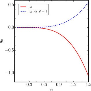
  , we will neglect the term involving D in (C12) and (C13). As an interesting example, we take Z = 1, i.e., β = 6. The expression (C12) becomes
Figure C1 gives an idea of the upper limit for the validity of the assumption  .
.
Figure C1. g0 and g2 for the case Z = 1, α = 1.76.
Download figure:
Standard image High-resolution image