

Abstract
The scrape-off layer (SOL) power fall-off length, λq, for parameters relevant to ASDEX Upgrade (AUG) L-mode discharges is examined by means of numerical simulations. The simulation data is acquired using synthetic probe data from turbulence simulations, which gives a high temporal resolution on the full density and pressure fields, required for an accurate evaluation of λq due to the strongly intermittent signals in the SOL. Electron conduction is found to dominate the parallel heat flux close to the separatrix, while ion convection dominates in the far SOL. Good agreement is found with the experimental scaling for AUG L-mode Sieglin et al (2016 Plasma Phys. Control. Fusion 58 055015), where λq is found to scale almost linearly with the safety factor, q, and to be weakly dependent on the power across the last-closed flux surface (LCFS), P. However, P depends on a wide range of parameters. In this paper we trace this dependence and the resulting fit of λq reveals a scaling proportional to the inverse square root of the electron temperature at the LCFS,  , and a linear dependence on q.
Export citation and abstract BibTeX RIS
1. Introduction
In magnetic confinement fusion devices most of the power across the last-closed flux surface (LCFS) is transported towards the divertor along magnetic field lines in a narrow region close to the separatrix [1]. The width of this channel is denoted as λq and it is crucial to know this parameter when determining the divertor peak heat load, which for ITER steady state operation needs to be kept below 10 MW m−2 due to material constraints. To estimate λq for ITER, several empirical scaling laws have been derived based on engineering parameters and extrapolated to ITER relevant parameters, both for limited plasmas [2–4] and for divertor plasmas [5–8].
The different scaling laws, however, do not all agree and it is not yet clear how much individual heat flux channels contribute to λq. In the experimental scaling laws, λq is either determined at the outer mid-plane using reciprocating Langmuir probes (as in [3]) or at the divertor using infra-red spectrometry and then mapping it to the outboard mid-plane (as in [1]). Neither of these methods provide insight into the individual contributions from electrons and ions to λq, and both are subject to large uncertainties when estimating λq and the corresponding parameters, e.g., when determining the position of the LCFS. For larger machines like AUG, it has been shown that the width of the parallel heat flux channel, λq, and the width of the parallel electron temperature channel, λTe, even when in L-Mode conditions, are well correlated by Spitzer–Härm conduction and hence λq/λTe = 2/7 is found [9, 10]. This correlation, however, is doubtful for smaller machines like TCV and Compass, so an experimental multi machine scaling for the power width in L-Mode conditions is difficult to establish and prone to artefacts; therefore this paper focuses on AUG L-mode relevant parameters. To identify the contributions from different heat flux channels to λq and to gain further understanding for the physical processes determining the scrape-off layer (SOL) power fall-off length, numerical simulations are employed. The advantage of simulations is that every parameter is known exactly, and thus contributions to λq can be identified and held up against experiments to validate the results. Several papers have investigated how λq scales with different parameters using numerical simulations [11–14], but these studies used either steady state transport codes or turbulence codes assuming cold ions. In the present paper we investigate the parameter dependence of λq by means of numerical simulations using the HESEL model [15], a 2D drift-fluid model. The model parametrises 3D dynamics with parallel heat fluxes and a sheath connection closure to incorporate the effects along the magnetic field lines as well as drift-wave terms in the region of closed field lines. Although this approach does not capture the full dynamics between the outboard mid-plane and the divertor, where full 3D codes such as HERMES [16], GBS [17] and TOKAM3X [18] are needed to incorporate these effects, the scaling found in this paper compares well with experimental results found for AUG L-mode [19]. Through turbulence simulations we deduce the parallel losses due to advection and conduction for both electrons and ions, and through parameter scans, with parameters chosen based on statistical significance using an approach similar to that in [3], we calculate numerical scalings for λq.
The outline of the paper is as follows; in section 2 we introduce the HESEL model used for the simulations and the methods used for calculating λq, in section 3 we present how the scaling parameters are chosen and the derived numerical scaling laws, and finally in section 4 we summarise and conclude the work.
2. The HESEL model
The HESEL model [15] is used for simulations throughout the paper. HESEL is a 2D model derived from the Braginskii two-fluid equations [20] solving for the density, n, generalised vorticity,  , electron pressure, pe and ion pressure, pi. 3D dynamics are parametrised following the approach and assumptions given in [21]. The simulations are conducted in a domain at the outboard mid-plane of a tokamak, as illustrated in figure 1. For all equations, Bohm normalisation has been imposed;
where Te is the electron temperature, Ti is the ion temperature, n is the density, φ is the electrostatic potential and t is time. The normalisation parameters are the ion cyclotron frequency,  , the ion gyroradius at electron temperature,
  , the electron charge, e, the reference electron temperature, Te0, the reference density, n0, the magnetic field strength at the outboard mid-plane, B0, the ion mass, mi, and the constant sound speed at the reference electron temperature,
  .
.
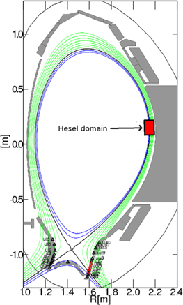
Figure 1. The cross-section of AUG with the HESEL domain indicated to scale by the red box.
Download figure:
Standard image High-resolution imageThe HESEL model reads


where  is a material derivative, with
  being the magnetic field modulus, R0 is the device major radius, a is the device minor radius, x is the radial coordinate from the LCFS and ∂t = ∂/∂t.
  denotes the material derivative with constant magnetic field.
  is the curvature operator, where
  is a unit vector in the direction of the magnetic field. The Poisson bracket is
The right-hand sides of equations (2)–(5) consist of perpendicular dissipation terms and parametrised parallel dynamics, given by
with the neoclassical diffusion coefficients given by
as derived in [21] where ρi0 is the ion gyroradius and ρe0 is the electron gyroradius, both at reference temperaures. νii0 is the ion–ion collision frequency at reference temperature, νei0 is the electron–ion collision frequency at reference temperature, q is the safety factor, and  , where Ti0 is a reference ion temperature. L∥ is the parallel connection length,
  is the Bohm potential and
  is the drift-wave coefficient. φs is the potential at the sheath entrance and Te,s is the electron temperature at the sheath entrance. In this paper we have assumed that the plasma is connected to the sheath, which is modelled using
  and φs = φ(x, y, t), i.e. the sheath dissipation depends on the full temperature and potential fields.
The term  is the energy transfer between electrons and ions. The tilde
  denotes a fluctuating term of the field f and
  denotes the poloidal average, defined as
where Ly is the poloidal length of the domain. At the inner boundary, the profiles are forced with the characteristic time τp towards prescribed profiles, np, pe,p, pi,p. τp is kept shorter than the interchange time, and the profiles are made to resemble typical profiles measured in the edge region of tokamak experiments and thus act as particle and energy sources, while avoiding unphysical steep gradients generated at the inner boundary when using constant particle and energy sources [15].
The parallel dynamics are parametrised in the form of parallel loss terms due to advection and electron and ion heat conduction (Spitzer–Härm conduction) with loss rates given by
where LB = qR0 is the parallel ballooning length.  is the electron (ion) thermal speed,
  is the electron-electron (ion–ion) collision frequency, both depending on the local values of
  so that
  and M is the parallel Mach number assumed to be M = 0.5 at the outboard mid-plane (see [22] for a thorough description of this assumption). Finally
  is the sound speed, which depends on the local electron and ion temperatures. We note that in order for Spitzer–Härm conduction to be valid, the electron collisionality [23]
which is fulfilled for all simulations in this paper.
2.1. Evaluation of λq
Assuming that the transport across the LCFS originates from ballooning-like turbulence in a poloidal extend of 60° at the outboard mid-plane [15], given approximately by 2πa/6 ≈ a, and assuming that the power is evenly distributed in this region, we can calculate the radial profile of the parallel heat fluxes. This is done using data from from synthetic probes in the HESEL domain illustrated in figure 2, where na, pa,e,i is the value of the fixed profile at the inner boundary for the density and the electron and ion pressures, respectively, and φa (see figure 2) is chosen so that ω* = 0 at the inner boundary.
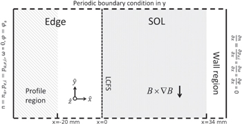
Figure 2. An illustration of the HESEL domain (not to scale) with boundary conditions and geometry illustrated in the plot.
Download figure:
Standard image High-resolution imageThe parallel heat flux at the outboard mid-plane is calculated from the parametrised parallel dynamics, and following the parametrisation stated in [21] as well as the contribution from the ion Spitzer–Härm conduction, we get four contributions to the parallel heat flux. The approach used in HESEL assumes quasineutrality, which consequently means that only small variation between the parallel velocities is allowed, and as a result, the thermal heat flux is assumed small compared to the other four contributions and has been neglected. The contributions to the parallel heat flux are thus a contribution from the electron advection, q∥,a,e, the ion advection, q∥,a,i, the electron conduction (also known as Spitzer–Härm conduction), q∥,SH,e and the ion conduction, q∥,SH,i, given by
where  denotes a temporal average. All terms are multiplied by the poloidal extent of the ballooning region, a, following the assumption above. We should state that macroscopic heat fluxes have been neglected since the mean fluid velocity at the outboard mid-plane is negligible. However, when approaching the divertor target, part of the thermal energy in expanding filaments will be converted to kinetic energy of the ions streaming toward the target plates at the filament fronts and this contribution to the heat flux would have to be evaluated. However, at the outboard mid-plane the parallel heat flux is described by the four contributions stated above. It is important to note that the full temperature and pressure fields are used for computing the parallel fluxes in equations (16) and (17). Since a significant fraction of the transport across the LCFS is intermittent [24], the parallel heat fluxes can not be calculated solely based on temporally averaged profiles, but need to be evaluated using the full temporal signals to capture the contributions from the intermittent bursts. To illustrate the importance of using the full fields, we have plotted the electron temperature at the LCFS in the poloidal centre of the domain as a function of time in figure 3(a). Here it is seen that the electron temperature is subject to large fluctuations varying by more than a factor of five. This inevitably influences the value of the parallel heat flux, as is illustrated in figure 3(b), where we have plotted the electron contributions to the parallel heat flux evaluated using equations (16) and (17) using the full fields (blue) and the temporally averaged fields (magenta). The difference is most pronounced in the Spitzer–Härm conduction, where the averaged profile leads to an estimation of the heat flux, which is a factor of two smaller at the LCFS than the profile found using the full fields.
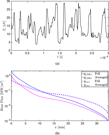
Figure 3. (a) Fluctuation level at the LCFS in the poloidal centre of the domain for a simulation with AUG relevant parameters. Only part of the temporal domain is shown. The full simulation is an order of magnitude longer. (b) The electron conduction (solid) and electron advection (dashed) contributions to the parallel heat flux for a typical simulation with AUG relevant parameters. The blue lines indicate the contributions calculated using the full fields and the magenta lines indicate the contributions calculated using averaged profiles.
Download figure:
Standard image High-resolution imageThe total parallel heat flux is the sum of all four contributions in equations (16) and (17), so

The SOL power fall-off length is then calculated as
where 0 is the location of the separatrix.
A typical heat flux profile for parameters relevant for ASDEX Upgrade is seen in figure 4. The four contributions to the total heat flux are illustrated in the plot, and as seen from the figure, the electron conduction dominates the parallel transport close to the LCFS, while the ion advection and electron advection become the dominant terms in the far SOL, where the ion conduction remains insignificant throughout the SOL. This is made more evident when looking at the ratio of the individual contributions with respect to the full heat flux profile as a function of the radial position, which is illustrated in figure 5. Here we see that the contribution from ion advection becomes dominant a few millimetres into the SOL. Note that the illustrated domain does not show the full simulation domain, but only depicts the SOL.

Figure 4. A typical parallel heat flux profile for AUG relevant parameters. The vertical lines indicate the 95% confidence limits on the averaged values.
Download figure:
Standard image High-resolution image
Figure 5. The fraction of the total heat flux for each of the four contributions. The dashed black line indicates the extent of the power fall-off length, λq, as calculated using equation (19).
Download figure:
Standard image High-resolution image3. Scrape-off layer power fall-off length
The simulations, from which the heat flux profiles are calculated are repeated scanning several AUG relevant L-mode parameters. This is done in order to derive a numerical scaling law for λq in L-mode. λq is calculated using equation (19) for every scanned parameter, and a fit of λq is made as a function of different combinations of parameters. The scans are performed by varying the parameters one at a time while all other parameters are kept fixed at typical AUG L-mode values, R0 = 1.65 m, a = 0.5 m, q = 4.5 and B0 = 1.9 T. Since the total power across the LCFS, P, and the LCFS values of n, Te and Ti are not input parameters, but depend on the forced profiles and the scanned input parameters, they vary slightly when the other parameters are scanned and they themselves are scanned by varying their respective forced profiles. The range of the scans are listed in table 1.
Table 1. The scaled parameters with corresponding ranges.
| Parameter | Units | Range |
|---|---|---|
| R0 | (m) | 1–5 |
| a | (m) | 0.3–1.2 |
| q | 3.8–9.0 | |
| B0 | (T) | 1.5–2.3 |
| P | (MW) | 0.04–1.27 |
| nLCFS |
![$[{10}^{19}\ {{\rm{m}}}^{3}]$](https://content.cld.iop.org/journals/0741-3335/60/8/085018/revision2/ppcfaace8bieqn24.gif)
|
1.1–2.8 |
| Te,LCFS | (eV) | 11–22 |
| Ti,LCFS | (eV) | 14–43 |
Here  is the total power across the LCFS, where the 2π(R0 + a) accounts for the circumference of the tokamak, nLCFS is the density at the LCFS and Te(i),LCFS is the electron(ion) temperature at the LCFS. We are aware that the electron and ion temperatures are low compared to usual AUG parameters, however, it should be noted that the LCFS is at the bottom of a steep gradient and moving the position 0.5 cm further in (which is less than the precision with which the position of the LCFS is determined in experiments) increases the temperatures by more than 50%.
3.1. Comparison with experimental scaling
First we investigate the experimental L-mode scaling from AUG derived in [19]. In this paper, a scan of P and q is performed, while the fit of B0 is taken from a study of an H-mode scaling at AUG in [5] and the parameter was thus not scanned in the paper. The scaling arrived at is given by

where B0 is not a scanned parameter.
In order to compare our numerical results with the experiments, we include scans with the same parameters as in [19]. This means that R0 = 1.65 m and a = 0.5 m are kept constant, while the variation in nLCFS is kept small using a range of  –
– . A fit is then made using

where a nonlinear fitting routine using an iterative least squares estimation (nlinfit in MATLAB) is used to determine the parameters A, b, c and d. λq,fit is plotted as a function of the numerically found value for λq in figure 6, where the best fit is found to be

We observe a fit with a coefficient of determination of R2 = 0.93. The fit is weakly dependent on the power across the last-closed flux surface, P, it scales almost linearly with the safety factor, q, and it is weakly dependent on the toroidal magnetic field, B0. Comparing this scaling to equation (20) we observe a match within the error bars on P and we observe the same trend with an almost linear dependence with q. The scaling with toroidal magnetic field, B0, differs between the two scalings, however, it should be noted that B0 was not a scaled parameter in [19], so the two scalings cannot be directly compared with respect to this parameter.
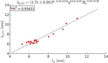
Figure 6. The nonlinear fit of λq with the parameters P, q and B0 plotted with respect to the numerically found λq, given by equation (19). Note that each dot corresponds to a separate simulation.
Download figure:
Standard image High-resolution image3.2. Choice of scaling parameters
The scaling in the previous section was derived in order to compare the results with the experimental scaling from AUG. This meant that the scanned parameters were limited to P, q and B0. Now, in order to make a more systematic investigation of the parameter dependence of λq, we fit it to all parameters listed in table 1. However, some of the parameters have strong mutual correlation, so, following the approach in [3], we calculate the correlation between the different parameters. Since the correlation coefficient describes a linear correlation between two quantities, we determine the coefficient by making a linear fit between the logarithms of the two parameters in question. The mutual correlation between each parameter is illustrated in table 2, and any parameters with a correlation of more than 50% are highlighted in bold face and are not included in the same scalings. We observe that the total power across the LCFS depends on a wide variety of scaling parameters, so in order to get a better understanding of what determines λq, it is fruitful to make a fit, where P is neglected and the other mutually independent parameters are included instead. Revisiting the scaling in equation (22) where P is replaced with the parameters nLCFS and Te,LCFS, we again apply the nonlinear fitting routine to get λq,fit. All parameter exponents in the fit are subject to uncertainties and are accompanied with 95% confidence intervals as calculated by the fitting routine. If the interval encompasses 0, then the parameter has no statistical significance and can be omitted from the scaling. When a parameter is omitted the fit is redone without this parameter and the process is repeated until only parameters with statistical significance remain. The outcome of this iterative routine is shown in table 3. We observe a very good fit with a coefficient of determination of R2 = 0.96 when including all parameters, which leads to a scaling given by
as illustrated in figure 7. However, we can, without significantly deteriorating the coefficient of determination, remove the parameters with the largest uncertainties, which is what we have done in the last two iterations in table 3. This leads to a simple scaling, where λq is solely determined by the electron temperature at the LCFS and the safety factor;

with a coefficient of determination of R2 = 0.95, which is plotted in figure 8. Comparing this fit, to figure 7, we do not observe any major improvements to the fit quality with more parameters. This means that the extra parameters in the fit in equation (23) compared to equation (24) merely add complexity, but do not significantly improve how well λq is described by the parameters.

Figure 7. The nonlinear fit λq with respect to the parameters nLCFS, q, B0 and Te,LCFS for simulations where P, q and B0 are scanned.
Download figure:
Standard image High-resolution image
Figure 8. The nonlinear fit λq with respect to the parameters Te,LCFS and q for simulations where P, q and B0 are scanned.
Download figure:
Standard image High-resolution imageTable 2. Mutual correlation between the logarithms of the different fitting parameters.
| Corr. (%) | a | nLCFS | q | Te,LCFS | Ti,LCFS | B0 | P | a/R0 |
|---|---|---|---|---|---|---|---|---|
| R0 | 63 | 24 | 0 | 49 | 19 | 1 | 71 | 0 |
| a | 24 | 0 | 35 | 15 | 1 | 79 | 9 | |
| nLCFS | 7 | 23 | 12 | 3 | 53 | 0 | ||
| q | 37 | 32 | 1 | 6 | 13 | |||
| Te,LCFS | 89 | 5 | 76 | 0 | ||||
| Ti,LCFS | 6 | 50 | 0 | |||||
| B0 | 5 | 0 | ||||||
| P | 0 |
Table 3. Scaling where P, q and B0 are scanned.
| A | nLCFS | q | B0 | Te,LCFS | R2 |
|---|---|---|---|---|---|
| 8.06 ± 2.14 | 0.54 ± 0.32 | 0.85 ± 0.07 | −0.20 ± 0.15 | −0.58 ± 0.11 | 0.96 |
| 6.16 ± 1.38 | — | 0.93 ± 0.05 | −0.28 ± 0.15 | −0.45 ± 0.08 | 0.96 |
| 5.02 ± 1.04 | — | 0.92 ± 0.05 | — | −0.44 ± 0.09 | 0.95 |
3.3. Scaling with nLCFS
The λq scalings found in equations (22) and (24) were derived with a scan over P, q and B0 to be able to compare with experimentally found values. However, we observed large uncertainties on the exponents of several parameters in the scalings, so in order to reduce the range of the confidence interval for the parameter exponents, a dedicated scan of nLCFS with the range given in table 1 was conducted and included in the λq fits. The nonlinear fitting routine described previously is applied with the extra parameter scan and the result is seen in table 4. We get a match within the error bars on all parameters compared to the fit in seen in equation (23). However, we still get large uncertainties on B0 and when removing this parameter from the scaling, as is done in the last step in table 4, we do not observe a significant reduction in the fit quality. This leads to a fit given by

with a coefficient of determination of R2 = 0.93. The fit is plotted in figure 9 and we observe that the points lie very close to the straight line indicating that λq is described well by the fourth root of nLCFS, which compares well with [6], the inverse square root of Te,LCFS and linearly with q.
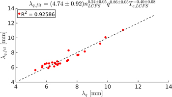
Figure 9. The nonlinear fit of λq with respect to the parameters nLCFS, q and Te,LCFS for simulations where P, q, B0 and nLCFS are scanned.
Download figure:
Standard image High-resolution imageTable 4. Scaling where P, q, B0 and nLCFS are scanned.
| A | nLCFS | q | B0 | Te,LCFS | R2 |
|---|---|---|---|---|---|
| 5.57 ± 1.28 | 0.23 ± 0.05 | 0.86 ± 0.05 | −0.23 ± 0.18 | −0.41 ± 0.08 | 0.93 |
| 4.74 ± 0.92 | 0.24 ± 0.05 | 0.86 ± 0.05 | — | −0.40 ± 0.08 | 0.93 |
3.4. Scaling with R0
Finally, we investigate the dependence of λq on the major radius, where all parameter scans from table 1 are included. R0 enters the calculations in a wide range of ways. First it enters in the curvature operator ∝1/R0, so a larger major radius decreases the amount of turbulence. The connection lengths and ballooning lengths are ∝R0 and the neoclassical corrections in the diffusivities are  . This means that the perpendicular diffusivities increase with R0, whereas the sheath loss and the other parallel losses decrease. It is therefore difficult to predict exactly how R0 will affect λq.
The parameter scan of R0 is conducted both with a fixed aspect ratio, a/R0 of 0.3, varying both a and R0 to keep the ratio fixed, and with a fixed minor radius of a = 0.5 m, so the aspect ratio varies between 0.1 and 0.3. The scaling is seen in table 5.
Table 5. Scaling where P, q, B0, nLCFS and R0 are scanned.
| A | nLCFS | q | B0 | Te,LCFS | R0 | R2 |
|---|---|---|---|---|---|---|
| 3.70 ± 1.04 | 0.27 ± 0.06 | 0.84 ± 0.07 | −0.21 ± 0.24 | −0.37 ± 0.10 | 0.64 ± 0.04 | 0.93 |
| 3.19 ± 0.72 | 0.27 ± 0.06 | 0.84 ± 0.07 | — | −0.36 ± 0.10 | 0.63 ± 0.04 | 0.93 |
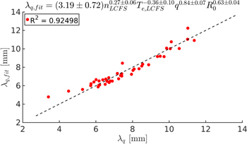
The best fit is found to be
with R2 = 0.93. As illustrated in figure 10, the fit is very close to the straight line with the exception of two outliers for very small major radii. This scaling with the major radius is in sharp contrast to what was found in the multi machine scaling in [5], where λq was found to be independent of the major radius, but agrees well with Halpern [8], Militello [13] and Myra [25]. The discrepancy with the experimental multi machine scaling may be attributed to the decrease in parallel losses with increasing major radius, which broadens λq. However, these parallel loss terms are 2D parametrisations of a 3D field, and therefore do not capture the dynamics between the outboard mid-plane and the divertor region, where the parallel heat flux is measured in [5]. In order to capture these dynamics and describe the heat flux at the divertor, a full 3D model will be necessary. The effects of such 3D models on filamentary transport are discussed in [26, 27] and the inclusion of 3D effects on the SOL width is discussed in [28].
Figure 10. The nonlinear fit of λq with respect to the parameters nLCFS, q, Te,LCFS and R0 for simulations where n, P, q, B0.
Download figure:
Standard image High-resolution image
4. Conclusion
In this paper, we have investigated the SOL power fall-off length, λq, by means of numerical simulations using the HESEL model. Since plasma transport in a tokamak is strongly intermittent, it is crucial to account for this intermittency when determining λq and averaged profiles can thus not be used. We have calculated the SOL power fall-off length by determining the parallel heat fluxes using full fields. Assuming that both advection and conduction for ions and electrons constitute the parallel heat flux, we get four individual contributions. We observe for typical AUG L-mode parameters, that electron conduction dominates the parallel heat flux close to the separatrix, but further into the SOL electron and ion advection take over, with the ion advection being dominant in the far SOL, and broaden λq, which is determined by the weighted average position of the parallel heat flux.
In order to compare with experimentally found scaling laws for λq, we initially made a parameter scan using parameters comparable to those used in AUG L-mode discharges. From this, we found a scaling law given by

which is close to the L-mode scaling in [19] with a weak dependence on the total power across the LCFS, P, and an almost linear dependence on the safety factor, q. The dependence on the toroidal magnetic field differs between the experimental and numerical scalings, but since it was not a scaled parameter in [19] we cannot compare the two.
The experimental scaling laws were derived on the basis of engineering parameters, which influence the properties of the plasma, but do not tell us much about the physical processes behind the SOL power fall-off length. To get a better understanding of what dictates λq, we examined the correlation between parameters which influence λq. It was found that P depends on a number of different parameters, so to understand what determines λq, the scaling was redone with P replaced by the density at the LCFS, nLCFS, and the electron temperature at the LCFS Te,LCFS. Here it was found that λq can be described by the two parameters q and Te,LCFS and that λq scales almost linearly with q and as one over the square root of Te,LCFS.
Moving on to include a wider range of scanned parameters, including a dedicated scan of nLCFS and the major radius, R0, revealed a dependence of λq on nLCFS and R0 in addition to the dependence on q and Te,LCFS. The best fit for λq was found to be

The dependence on R0 conflicts with what was found in [5], where λq was found to be independent of R0. Since the major radius enters the HESEL model both in the parallel loss terms, the diffusivities and in the curvature operator, it is not straightforward to determine which term this inconsistency arises from and this analysis is therefore left for future studies.
Despite this we do observe a good fit with the experimental L-mode scaling for AUG, and we believe that the λq scalings we have found in this paper can act as a guideline for future experiments. In all scaling laws derived in this paper, it is important to note that the theory used is only valid for strongly collisional plasmas. The extrapolation of λq to ITER, however, needs to be done with care, since ITER is not expected to be dominated by Spitzer–Härm conduction due to it operating in a low collisional regime.
Acknowledgments
This work has been carried out within the framework of the EUROfusion Consortium and has received funding from the Euratom research and training programme 2014–2018 under grant agreement No. 633053. The views and opinions expressed herein do not necessarily reflect those of the European Commission.