
Abstract
Objective. Multi-parametric magnetic resonance imaging (mpMRI) has become an important tool for the detection of prostate cancer in the past two decades. Despite the high sensitivity of MRI for tissue characterization, it often suffers from a lack of specificity. Several well-established pre-processing tools are publicly available for improving image quality and removing both intra- and inter-patient variability in order to increase the diagnostic accuracy of MRI. To date, most of these pre-processing tools have largely been assessed individually. In this study we present a systematic evaluation of a multi-step mpMRI pre-processing pipeline to automate tumor localization within the prostate using a previously trained model. Approach. The study was conducted on 31 treatment-naïve prostate cancer patients with a PI-RADS-v2 compliant mpMRI examination. Multiple methods were compared for each pre-processing step: (1) bias field correction, (2) normalization, and (3) deformable multi-modal registration. Optimal parameter values were estimated for each step on the basis of relevant individual metrics. Tumor localization was then carried out via a model-based approach that takes both mpMRI and prior clinical knowledge features as input. A sequential optimization approach was adopted for determining the optimal parameters and techniques in each step of the pipeline. Main results. The application of bias field correction alone increased the accuracy of tumor localization (area under the curve (AUC) = 0.77; p-value = 0.004) over unprocessed data (AUC = 0.74). Adding normalization to the pre-processing pipeline further improved diagnostic accuracy of the model to an AUC of 0.85 (p-value = 0.000 12). Multi-modal registration of apparent diffusion coefficient images to T2-weighted images improved the alignment of tumor locations in all but one patient, resulting in a slight decrease in accuracy (AUC = 0.84; p-value = 0.30). Significance. Overall, our findings suggest that the combined effect of multiple pre-processing steps with optimal values has the ability to improve the quantitative classification of prostate cancer using mpMRI. Clinical trials: NCT03378856 and NCT03367702.
Export citation and abstract BibTeX RIS

Original content from this work may be used under the terms of the Creative Commons Attribution 4.0 licence. Any further distribution of this work must maintain attribution to the author(s) and the title of the work, journal citation and DOI.
1. Introduction
Prostate cancer (PCa) is one of the most commonly diagnosed cancers in men worldwide and is the third leading cause of cancer-related death in North America (Yoo et al 2019). Accepted methods for the detection of clinically significant PCa include some combination of the prostate-specific antigen (PSA) test, digital rectal exam, and magnetic resonance imaging (MRI). Since PSA is not specific to PCa, an increase in PSA screening has led to overdiagnosis and unnecessary biopsies in men with low risk of developing clinically significant PCa. MRI is thus becoming an increasingly useful tool in the characterization of PCa (Ahmed et al 2017).
Multi-parametric magnetic resonance imaging (mpMRI) is a combination of structural and functional imaging techniques (T2-weighted (T2w) imaging, diffusion-weighted imaging (DWI), and dynamic contrast-enhanced (DCE) MRI) that has found an increasingly prominent role in detection, treatment, and prognosis of PCa. Its high sensitivity for the detection of microstructural tissue alterations lends itself well to the localization of prostate tumors (Turkbey et al 2010, Delongchamps et al 2011). This is particularly relevant in radiotherapy where recent advancements in dose delivery techniques require increasingly higher levels of precision. Tumor-dose escalated radiotherapy is one such treatment option that has emerged as a promising strategy for improving patient outcomes (Kerkmeijer et al 2021), highlighting the importance of accurately delineating tumor targets.
Despite the sensitivity of mpMRI in the localization of prostate tumors, it is hindered by a lack of specificity in the presence of benign conditions that mimic the image properties of cancerous tissue. PCa is characterized by low signal intensity in T2w images, but a hypointense signal may also be indicative of benign prostatic hyperplasia (BPH), prostatitis, or post-biopsy hemorrhage (Ikonen et al 2001). The hypointense signal of the apparent diffusion coefficient (ADC), calculated from two high b-value DW images, that is characteristic of cancerous tissue may also be confounded by prostatitis and BPH, though the signal is not typically as low as that for PCa. Moreover, both prostatitis and BPH have been shown to mimic tumors on DCE MRI through increased perfusion and vascularity (Verma et al 2012). Additional confounds include atrophy, fibrosis, calcification, necrosis, and cysts. The presence of such benign conditions may thus lead to inaccuracies in the identification and characterization of PCa by mpMRI.
The impact of these benign confounds can be especially detrimental to the quantitative classification of PCa using tumor localization models. These models extract quantitative features from mpMRI with the underlying assumption that any differences between voxel values are due solely to the presence or absence of PCa. In order to reduce the effect of benign confounds and thereby improve tumor localization based on mpMRI, Dinh et al (2017) proposed a model that included two sources of prior knowledge: a population-based tumor probability atlas (Ou et al 2009) and a patient-specific map based on clinical information obtained from a TRUS-guided procedure. While the addition of prior knowledge features to mpMRI-based features was shown to improve tumor localization, there is still room for improvement, given the variety of confounds that may be present, as well as the variability of mpMRI that is known to occur both within and across patients.
The ability of mpMRI to provide robust, reliable information that can be used to adequately assess tissue properties can be strengthened by standardizing its use across sites and institutions. Image pre-processing, for example, is a crucial step for any MRI analysis and is well-known for its role in the removal of artifacts and intensity variations that can lead to improved image quality and, thereby, result in more robust quantitative MRI feature extraction.
The number and type of pre-processing steps that may be applied to mpMRI of the prostate prior to any quantitative analysis, however, is quite diverse (Lemaître et al 2015). The decisions regarding which, if any, pre-processing steps to use often depend on multiple factors, such as image acquisition protocols, the image modalities that will be included, the cohort size, the quantitative analysis to be performed, or the pre-processing tools available. Given the vast number of pre-processing pipelines that this myriad of options could engender, it is important to consciously assess not only individual pre-processing elements, but also the effect that successive steps of an entire pre-processing pipeline may have. Previous studies have, for instance, investigated the effects of various methods of bias field correction and intensity normalization on T2w images of the prostate (Viswanath et al 2011, Isaksson et al 2020, Scalco et al 2020). It has been demonstrated, however, that an appreciable interaction exists between these two pre-processing steps. It is recommended, for example, that bias field correction should be performed before intensity normalization in order to prevent the introduction of additional intensity non-standardness (Madabhushi and Udupa 2005). Moreover, bias field correction has been shown to improve image registration quality by mitigating the effect in intensity inhomogeneities within the images that may adversely affect the accuracy of intensity-based registration algorithms. In light of these considerations, the development of an entire standardized pre-processing pipeline has the potential to improve upon the classification of PCa in mpMRI over the optimization of individual steps alone.
In this study we evaluate the combined effect of bias field correction and normalization on T2w images, as well as the registration of DW to T2w images (figure 1). We assess the results by considering both individual and application-specific metrics. Specifically, we examine the impact of each successive component of the pre-processing pipeline on the accuracy of tumor probability maps generated from the prior knowledge-based model. Irregularities in the intensity values of mpMRI due to the presence of artifacts and geometrical distortions may occur in both healthy and tumor tissue, thereby leading to false positives and false negatives in tumor localization. Thus, the evaluation of mpMRI by both individual metrics and application-specific metrics is relevant to healthy and tumor tissue alike. As such, we perform a systematic evaluation of each pre-processing step and determine whether these lead to an improvement in the ability of mpMRI to distinguish healthy tissue from suspected PCa.
2. Materials and methods
2.1. Clinical data
This study is based on 31 PCa patients from a single institution enrolled in a prospective, research ethics board approved clinical trial (NCT03378856 and NCT03367702). This research was approved by Comité d'éthique du CHUM, No 17.032 and 17.244. The research was conducted in accordance with the principles embodied in the Declaration of Helsinki, as well as in accordance with local statutory requirements. All participants gave written informed consent to participate in the study. Written informed consent was also given for publication by all participants.
Multi-parametric imaging consisting of a T2w (TR = 3377 ms, TE = 80 ms, FOV = 0.185 × 0.185 × 4.5 mm3), diffusion-weighted imaging (DWI) (TR = 3280 ms, TE = 79 ms, FOV = 1.774 × 1.774 × 4.5 mm3, b-values = 0–2000 s mm−2), and dynamic contrast-enhanced (DCE) (TR = 5.76 ms, TE = 0 ms, FOV = 0.917 × 0.917 × 3.0 mm3, dynamic scan time = 15.55 s, scan duration = 311 s, contrast agent = ProHance (gadoteridol, Bracco Imaging), dose = 0.2 cc kg = up to maximum of 20 cc, injection rate = 2 cc s−1) compliant with PI-RADS v2.1 (Weinreb et al 2016, Turkbey et al 2019) was performed on a 3 T MRI scanner (Philips Ingenia) prior to radiotherapy.
2.2. mpMRI preparation
A genitourinary radiation oncologist manually delineated contours of the prostate, peripheral zone (PZ), and tumors in both the PZ and transition zone (TZ) with a PI-RADS score of 4 or 5 via the aid of institutional PI-RADS reports. ADC maps were computed from three b-value DW images (b = 50, 600, 800 s mm−2) using the scanner proprietary software. Ktrans maps were derived from the DCE-MRI images according to the generalized kinetic model (Tofts et al 1999). A population-based arterial input function (Parker et al 2006) was used to generate Ktrans maps after adjusting the functional form to fit the temporal features of this dataset. In the absence of a pre-contrast T1 acquisition, a constant value of 1597 ms was used (Fennessy et al 2012). Ktrans generation was performed using the PkModeling module in 3D Slicer (v 4.10.1) (http://slicer.org) (Fedorov et al 2012). Ktrans images were normalized according to the median value in the PZ. The ADC images and Ktrans images were resampled to a voxel size of 0.19 × 0.19 × 4.5 mm3 to match the resolution of the T2w images. ADC images were not resampled when performing multi-modal deformable registration to the T2w images. No motion correction was performed prior to ADC or Ktrans image generation.

Figure 1. Full pre-processing pipeline including all three steps: (1) bias field correction, (2) intensity normalization, and (3) deformable registration.
Download figure:
Standard image High-resolution image2.3. Pre-processing optimization
Prior to the application of each pre-processing step, optimal parameter options were determined for each potential method. Each parameter option was initially set to the default or recommended value for a given method. A range of values were then tested for each parameter option individually while keeping all other parameters at the default or recommended settings. The performance of a particular parameter option was then evaluated by one or more of the relevant individual metrics for that pre-processing method. Once all parameter options were determined, a final implementation of each method was carried out using these optimal parameter values. The performance of this implementation was assessed by all relevant individual metrics, as well as the application-specific task of tumor localization, since the performance of a pre-processing tool has been shown to vary according to the individual metric used for evaluation (Viswanath et al 2011, Rohlfing 2012). Where applicable, results for the individual metrics are represented by violin plots, which are a combination of a box plot and a kernel density plot. As such, they display both summary statistics and the density of the variable. Like a box plot, the white dot depicts the median, and the thick gray bar shows the interquartile range. In addition, the thin gray line represents the distribution of the variable. Either side of the line is a kernel density estimation in which wider sections correspond to a higher probability of a given value, and narrow sections correspond to a lower probability of that value.
2.4. Bias field correction
MR images are often susceptible to intensity non-uniformity artifacts. These artifacts may occur as a result of inhomogeneities in the radio frequency field, eddy currents, or attributes that are inherent to the particular biological sample being imaged. The effect of the bias field manifests as a nonlinear, smooth variation of signal intensity values across the image. The result is an image for which intensity values of a given tissue type may vary with location in the image. This spatial invariance has been shown to adversely affect image processing algorithms for performing tasks such as segmentation (Li et al 2014), registration (Xu et al 2013), and classification (Li et al 2009), among others.
The aim of bias field correction is thus to remove this intensity inhomogeneity, and numerous methods have been proposed. We chose to explore the more commonly used retrospective models, so intensity inhomogeneity in the T2w images was therefore corrected using two well-established, publicly available methods: N4 (v 2.2.0) (Tustison et al 2010) and PABIC (v 1.0) (Styner 2000). Optimal parameter settings were first determined for each method by testing a range of values for each available parameter option, including number of iterations, shrink factors, and order. The number of iterations refers to the maximum number of iterations that the algorithm is run and is employed as at least one of the stopping conditions for the algorithm. In general, a higher number of iterations can produce a more reliable result, though this will increase the runtime. A shrink factor refers to a parameter that is associated with a multi-resolution implementation of the algorithm; in this approach, the amount of data to process is reduced by initially running the algorithm on a coarse resolution of the data. In addition to data reduction, the number of local minimums/maximums that could potentially confound the performance of the algorithm is also reduced. Fine detail is then gradually added to the image by gradually increasing the image resolution at subsequent levels of the multi-resolution approach. The shrink factor is the degree to which the image is downsampled at each resolution level. The order parameter refers to the order of the b-spline in the case of N4 and to the order of the Legendre polynomials in the case of PABIC. Additional parameters that are specific to N4 consisted of the mesh grid resolution, number of histogram bins, Wiener noise, and full width at half maximum (FWHM). As for PABIC, the initial step size, as well as the mutation factors cgrow and cshrink, were also optimized.
The performance of each parameter setting was evaluated individually using three commonly employed measures of the effects of bias field correction: the percent coefficient of variation (CoV), entropy, and the coefficient of joint variation (CJV). The CoV is expressed as a quotient between the standard deviation and mean of a given tissue class, t:

where t represents the whole prostate gland. The CJV takes two tissue classes into account, which in our case consisted of the central gland (CG) and PZ:
Each of these metrics should exhibit decreased values for bias field-corrected images. Moreover, the intensity inhomogeneity that occurs as a result of the bias field is thought to raise the entropy of the image data distribution. Entropy can be described as:
where G represents the total number of unique gray level intensities  in the region of interest (ROI) and
  is the probability of occurrence associated with each
  Thus, the entropy of bias field-corrected images should also decrease. The final implementation of each bias field correction method was then performed using a combination of all optimal parameter settings.
2.5. Intensity normalization
One well-recognized limitation of MR images is the lack of tissue-specific meaning in intensity values. This can lead to a drift in intensity values across both inter- and intra-patient acquisitions. Normalization aims to correct this drift by standardizing the intensity values across a dataset and is typically performed by one of three methods: centering the image intensity range according to its mean value, normalization of gray level values according to a specific ROI, and transformation of the histogram of the image to a reference intensity distribution. We refer to these methods as basic normalization, ROI normalization, and histogram matching normalization, respectively. Basic normalization refers here to z-score normalization. ROI normalization was performed by dividing all intensities by the median value in the PZ. Histogram matching normalization was implemented according to the method introduced by Nyú and Udupa (1999). This approach consists of two steps: (1) a training stage in which the landmarks of a standard histogram are determined from a training set of images and (2) transformation of each image histogram to the standard histogram. All bias field-corrected T2w images were included in the training step. A value of 4095 was chosen for s2, and quartiles were chosen as histogram landmarks. The bias field-corrected T2w images were thus normalized according to each of these techniques. The performance of each normalization method was assessed with the CoV, which is routinely used to evaluate this type of pre-processing task.
2.6. Deformable registration
Image distortion on DWI of the prostate due to chemical shift and susceptibility artifacts is a well-recognized phenomenon (Donato et al 2014, Hao et al 2017). Such distortions manifest as either local stretching or compression in the acquired image (Gallichan et al 2010). As a result, rigid registration is insufficient for the correction of local distortions on prostate DWI (Giannini et al 2015). Non-rigid registration, then, is often employed for more accurate alignment of T2w- and DW-images of the prostate (Buerger et al 2015). Thus, multi-modal deformable registration of the ADC image to the T2w image, representing the last step before a tumor map generation, was carried out using three popular, open source toolkits: elastix (Klein et al 2010), NiftyReg (Modat et al 2014), and ANTs (Avants et al 2011). In order to compare the performance of each toolkit, the same registration approach was followed. The registration of DW images is typically performed using non-rigid registration due to local deformations in these images that occur as a result of motion and susceptibility artifacts. In view of this, an intensity-based, non-rigid registration method that employs cubic b-splines to parameterize the deformation field was adopted as this has been shown to be a relatively simple, robust approach for both mono- and multi-modal implementations. The images were first aligned using an initial translation and then underwent a global transformation (rigid + affine). Non-rigid registration was then carried out by means of free-form deformation that utilizes a standard gradient-based optimization of cubic b-splines with mutual information as the similarity metric. Common parameter manipulations, including number of resolution levels, maximum number of iterations, interpolation order, number of samples, degree of smoothing, and regularization weight, were initially assessed using the Dice similarity coefficient (DSC) to measure the overlap of prostate gland delineations before performing the final registrations using optimal parameter values. The DSC is defined as follows:
where A and B represent the segmentations of the T2w image and ADC image, respectively. The registrations were first estimated between T2w and b = 0 (b0) images, and the resulting transformation was then applied to the ADC images. While the fundamental structure of this approach is the same for each of the three toolkits, the algorithmic implementations differ, potentially resulting in disparities in registration outcomes. The quality of registration for each toolkit was evaluated by three different metrics: (1) a tissue overlap measure represented by the DSC, (2) a deformation field assessment represented by the determinant of the Jacobian, and (3) the mean target registration error (TRE). The calculation of the TRE was based on natural landmarks identified in both the T2w and ADC images, such as BPH nodules or calcifications. The TRE was computed as the distance between the geometric centers of corresponding landmarks in the T2w and ADC images after registration.
2.7. Tumor probability map generation
Once the pre-processing steps were evaluated, tumor probability maps were generated using a previously developed tumor localization model that was trained on mpMRI data acquired on both Siemens and Philips scanners (Dinh et al 2017). The aim of this model is to reduce the number of false positive results by combining mpMRI features with prior knowledge features. A total of 31 features are extracted per voxel, which include 29 mpMRI features (3 intensity, 24 texture, and 2 blobness), one from a population-based tumor probability atlas (Ou et al 2009), and one from a map constructed from the biopsy report for that patient. Processing of all mpMRI and prior knowledge data before feature extraction is summarized in figure 2. The mpMRI features were extracted from the T2w, ADC, and Ktrans images according to the methods presented in Dinh et al (2017). Multi-parametric MRI-based features included both intensity and texture features. Texture features followed those proposed by Litjens et al (2014) and Vos et al (2012). Gaussian derivatives up to second order were extracted from the T2w images at exponentially increasing scales (σ = 1.5, 2.4, 3.8 and 6.0 mm). As for the ADC and Ktrans images, normalized multiscale blobness features (Lindeberg 1998) were computed over the same four scales. The first element of prior information is a population-based tumor probability atlas presented by Ou et al (2009). The tumor probability atlas consists of voxels that correspond to the number of specimens that contained a tumor at that voxel. The tumor probability atlas was registered to the T2w images using the non-rigid registration algorithm implemented with elastix. The second element of prior knowledge is a biopsy map that was constructed using a detailed biopsy scheme in which the prostate was divided into six regions: apex, middle, base, and left/right. Each voxel value in the biopsy map was assigned a value of zero or one, depending on whether or not a positive biopsy was reported in that location (1 = positive). Once constructed, the biopsy map was smoothed by convolving it with a Gaussian kernel (σ = 4.5 mm).
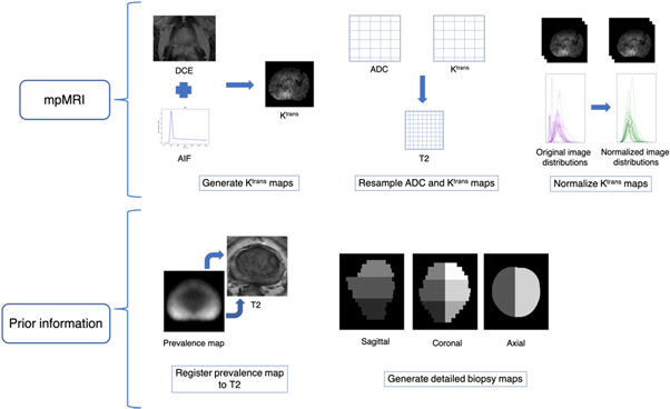
Figure 2. Workflow of data processing steps of the tumor localization model prior to feature extraction.
Download figure:
Standard image High-resolution imageThe tumor localization model was previously created and trained by Dinh et al (2017). Prostatectomy specimens obtained from each patient after mpMRI acquisition were used to establish ground truth tumor locations in a training cohort of patients. Slices of the prostatectomy specimens were stained with hematoxylin and eosin (H&E) and then registered to the T2w images. Each voxel of the training cohort was labeled as healthy or tumor tissue according to delineations on the H&E-stained slices by a pathologist. The aforementioned 31 features were then extracted for each voxel, and a logistic regression model was fitted to the histologic data obtained from the training cohort of patients according to Dinh et al (2017). The logistic regression function can be expressed as follows:
where  is the probability that a voxel
  belongs to a tumor,
  is the value of feature
 is the regression coefficient of feature
  and
and  is the offset. The model was validated in both a single-center and cross-center setting. Training and testing datasets for the single-center setting were established using a leave-one-out cross-validation approach. All patients were used to fit the model for the cross-center validation.
The classification model presented by Dinh et al (2017) was used here as presented in that study without any modifications to the model. The only difference is that instead of using non pre-processed imaging data, we are using pre-processed data as an input for testing the model in order to assess the effect of pre-processing on tumor classification accuracy. The pre-trained model was then used to generate tumor probability maps for four pre-processing variations: no pre-processing, bias field correction alone, bias field correction followed by normalization, and bias field correction and normalization followed by registration. The resultant tumor probability maps were evaluated by comparison with manually contoured tumors using the area under the curve (AUC). A Wilcoxon signed-rank test was performed with Bonferroni multiple comparison correction to determine whether tumor localization results differed significantly between various combinations of pre-processing steps (table 5). As four tests were performed in this study, the new significant p-value after Bonferroni correction is 1.25 × 10⁻².
To test the generalizability of this approach, the 31 patients were randomly divided into a training cohort of 20 patients and a testing cohort of 11 patients. We then repeated the entire analysis by first estimating the optimal parameter values for each pre-processing step on the training cohort and applying those pre-processing steps to the testing cohort. We then generated tumor probability maps on the testing cohort for each of the four pre-processing variations and evaluated the results using the AUC.
2.8. Feature evaluation
Clinically significant PCa has a characteristic appearance on mpMRI. In general, it is hypointense to surrounding tissue on T2w images and has an 'erased charcoal' appearance in the TZ. Likewise, since PCa is known to restrict diffusion, it also appears as hypointense on ADC images. The intensity values of PCa on DCE images, on the other hand, are expected to exhibit early enhancement, which manifests itself as hyperintense signal compared to healthy tissue. Image artifacts present on mpMRI can thus impact the expected appearance of PCa and ultimately affect any features that are extracted. Intensity inhomogeneities and intensity drift may lead to irregularities in intensity values that are not representative of the underlying tissue. This can affect both healthy and tumor tissue alike, resulting, for example, in healthy tissue that is more hypointense or tumor tissue that is more hyperintense than it should be. A tumor classification model that includes intensity value features may then be more prone to false positives and false negatives as a result if these artifacts are not mitigated.
Texture features that aim to characterize spatial patterns of image intensity can also be affected by the presence of unwanted artifacts. Materka and Strzelecki (2013) note that these features are susceptible to intensity inhomogeneities that require bias field correction. Moreover, it has also been shown that texture features depend not only on texture, but also on the mean and variance within an ROI. Thus, these features are also susceptible to intensity drift, and normalization is necessary to ensure that accurate texture features are calculated.
In order to assess the impact of each pre-processing step on the features extracted from mpMRI, we compared the value of each of the features, both within healthy tissue and in the suspected tumor, for each pre-processing step to the corresponding values in the non pre-processed images using the concordance correlation coefficient (CCC) (Isaksson et al 2020). The CCC is a measure of reproducibility between two sets x and y and is expressed as
where  is the standard deviation,
  is the mean, and
  is the covariance. The features evaluated with the CCC included only those extracted from the T2w and ADC images because only those are affected by the pre-processing steps. They included the T2w and ADC intensity values, the 24 texture features extracted from the T2w images, and the blobness feature calculated for the ADC images.
3. Results
3.1. Bias field correction
The optimal parameter values for each bias field correction method are shown in table 1. Of all the parameters available for N4, only the value of the spline order is equal to the default value. All of the optimized values for the PABIC parameters differ from the default values. The bias field correction applied to the T2w images improved image quality when compared to unprocessed images, but the results varied according to each method and the individual metrics used for evaluation (figure 3). N4 achieved the lowest value for CoV and entropy while PABIC marginally outperformed those images corrected with N4 when considering the CJV. In order to assess the benefit of bias field correction within the context of tumor localization, tumor probability maps were generated using T2w images corrected with either N4 or PABIC. Tumor classification performance in terms of the AUC was highest using PABIC bias field correction, whereas classification using N4 was equivalent to that of the T2w images before any bias field correction (table 2). As a result, PABIC was the bias field correction method selected for this study. A closer inspection of the effect of bias field correction on tumor localization showed that removal of the bias field led to intensity values that more accurately characterized PCa, i.e. an increase in true positive values in the tumor probability maps (figure 4).
Table 1. Optimized parameter values for N4 and PABIC.
| Parameter | N4 value | PABIC value |
|---|---|---|
| Number of iterations | 500 | 2000 |
| Shrink factor | 1 | 4 |
| Spline order | 3 a | NA |
| Initial mesh resolution | 4 | NA |
| FWHM | 0.25 | NA |
| Wiener noise | 0.05 | NA |
| Number of histogram bins | 150 | NA |
| Legendre polynomial order | NA | 2 |
| Initial step size | NA | 1.1 |
| cgrow | NA | 1.08 |
| cshrink | NA | 0.98 |
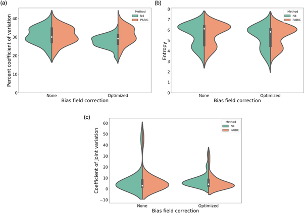
Figure 3. Bias field correction performance in terms of individual metrics (a) percent coefficient of variation, (b) entropy, and (c) coefficient of joint variation.
Download figure:
Standard image High-resolution imageTable 2. Pre-processing performance in terms of tumor localization. Bold values represent best accuracy scores.
| Pre-processing step | Tool | AUC |
|---|---|---|
| Bias field correction | None | 0.74 ± 0.11 |
| N4 | 0.74 ± 0.12 | |
| PABIC | 0.77 ± 0.11 | |
| Normalization | Basic | 0.85 ± 0.11 |
| ROI | 0.84 ± 0.10 | |
| Histogram matching | 0.85 ± 0.11 | |
| Registration | elastix | 0.84 ± 0.12 |
| NiftyReg | 0.81 ± 0.16 | |
| ANTs | 0.83 ± 0.12 |
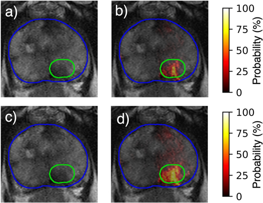
Figure 4. Comparison of (a) uncorrected T2w image and (b) resultant tumor probability map to (c) T2w image corrected with PABIC and (d) associated tumor probability map.
Download figure:
Standard image High-resolution image3.2. Intensity normalization
After bias field correction with PABIC, each of the three normalization methods was applied to the T2w images. Neither basic nor ROI normalization achieved a CoV value less than that achieved by PABIC alone (figure 5). Histogram matching normalization, however, did minimize the CoV, by comparison. While all three methods led to an improvement in tumor localization compared to bias field correction alone, basic and histogram matching normalization slightly outperformed ROI normalization in terms of the AUC (table 2). Histogram matching was thus chosen as the method for normalization as it was found to score best for both the CoV and tumor localization. In general, bias field-corrected images that were normalized according to the histogram matching technique demonstrated a slight reduction in the likelihood of false positives present in tumor probability maps generated on T2w images that had only been corrected using PABIC, though the difference was not substantial (figure 6).

Figure 5. Assessment of normalization methods in terms of individual metric CoV.
Download figure:
Standard image High-resolution image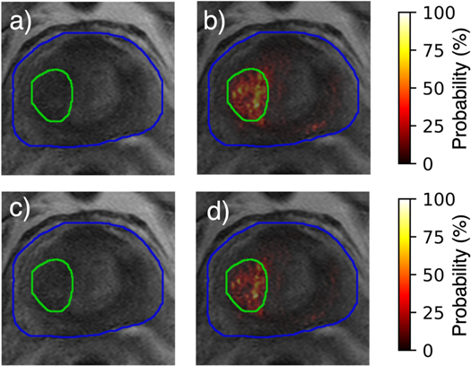
Figure 6. Effect of (a) PABIC-corrected T2w image with (b) subsequently generated tumor probability map in relation to (c) PABIC-corrected T2w image normalized using histogram matching and (d) resultant tumor probability map.
Download figure:
Standard image High-resolution image3.3. Deformable registration
Identical parameter options were assessed for each registration method where available. The resulting optimal values are given in table 3. Of the three methods, NiftyReg adhered most closely to the default or recommended values. All methods performed best at a single resolution level with no smoothing while both elastix and NiftyReg achieved the highest DSC value for a regularization weight of 0.05. All other parameter values differed according to the method used for registration. DSC values demonstrated an improvement in registration quality for elastix when compared to NiftyReg and ANTs (figure 7). The mean range of Jacobian determinant values over all subjects showed that elastix is the only method within the acceptable range of zero to slightly more than one (table 4). The mean TRE values, however, showed that NiftyReg attained a higher registration quality over elastix and ANTs. Tumor localization performance, though, was greatest for elastix compared to NiftyReg and ANTs (table 2). Thus, elastix was ultimately chosen as the preferred method for registration of the ADC images to the T2w images. When successful, this registration improved alignment of the tumor location across modalities and thereby improved the accuracy of the tumor localization model in that region (figure 8). Registration of the ADC using elastix resulted in poor alignment with the T2w image for a single patient (figure 9). In this case, the bladder of the ADC image was improperly aligned with the prostate gland of the T2w image, which resulted in misidentification of the tumor in the resultant probability map. Removal of this patient led to an increase in the AUC to a value of 0.87, though the result was still not significant (table 5). Tumor probability results for all three cases are shown in (see figures S1–S3 in supplementary materials).
Table 3. Optimized parameter values for each registration method.
| Registration | Multi-resolution (levels) | Maximum Iterations | Interpolation order | Samples (voxels) | Smoothing (mm) | Grid spacing (mm) | Regularization (weight) |
|---|---|---|---|---|---|---|---|
| elastix | 1 | 2000 | 1 | 2000 | 0 | 1 | 0.05 |
| NiftyReg | 1 | 300 a | 3 a | NA | 0 a | 5 | 0.05 |
| ANTs | 1 | 100 | 2 | 10% a | 0 | 1 | NA |
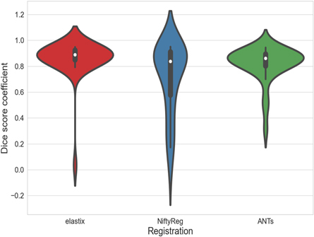
Figure 7. Performance of each registration method as measured by the Dice similarity coefficient.
Download figure:
Standard image High-resolution imageTable 4. Assessment of multi-modal registration by two individual metrics: Jacobian determinant and mean TRE. Bold values represent best metric scores.
| Registration | Jacobian determinant range | TRE (mm) |
|---|---|---|
| elastix | 0.44–1.69 | 12.01 ± 21.72 |
| NiftyReg | 7.56–9.29 | 6.57 ± 4.21 |
| ANTs | 0–7384.30 | 8.32 ± 4.59 |
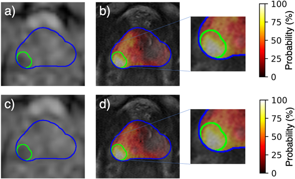
Figure 8. (a) Resampled ADC image and corresponding (b) tumor probability map compared to (c) ADC image registered using elastix and (d) associated tumor probability map.
Download figure:
Standard image High-resolution image
Figure 9. Failed registration for a single patient using elastix. (a) Resampled ADC image and (b) subsequently generated tumor probability map compared to (c) poor registration of ADC using elastix and (d) resultant tumor probability map.
Download figure:
Standard image High-resolution imageTable 5. Tests performed in this study along with the corresponding p-values. Bold values represent significant results (p-value = 1.25 × 10⁻²).
| Experiment | p-value |
|---|---|
| No pre-processing versus bias field correction alone | 4 × 10⁻³ |
| Bias field correction alone versus bias field correction with normalization | 1.2 × 10⁻⁴ |
| Bias field correction with normalization versus whole pre-processing pipeline | 3 × 10⁻¹ |
| Bias field correction with normalization versus whole pre-processing pipeline with removal of patient with poor registration | 4.4 × 10⁻¹ |
3.4. Tumor localization using complete pipeline
When considering the cumulative effect of multiple pre-processing steps, the application of bias field correction along with normalization achieved the highest level of tumor localization performance, followed closely by the full pipeline of bias field correction, normalization, and registration (figure 10). In general, the application of these pre-processing steps improves tumor localization by increasing the number of true positive results, as well as reducing the number of false positives. This improvement is greater for tumors located within the PZ compared to those in the TZ (figure 11), which are traditionally more difficult to identify. Similar results were obtained for the analysis of the generalizability of using an optimized pre-processing pipeline to improve tumor localization accuracy (see S5–S13 in supplementary materials).
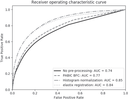
Figure 10. Performance of the tumor localization model in the classification of PCa for each pre-processing combination. Each combination listed includes the specified pre-processing step, as well as those preceding it, e.g. the elastix registration curve represents the accuracy of the tumor localization model for mpMRI that was bias field corrected, normalized, and registered.
Download figure:
Standard image High-resolution image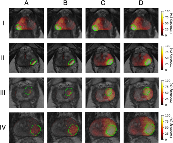
Figure 11. Tumor probability maps for four patients (rows) across all pre-processing combinations: (A) None, (B) PABIC bias field correction, (C) PABIC bias field correction + histogram matching normalization, and (D) PABIC bias field correction + histogram matching normalization + elastix registration. Tumors are located in the PZ for patients I and II and in the TZ for patients III. The tumor is located in the PZ and part of the TZ for patient IV.
Download figure:
Standard image High-resolution image3.5. Feature evaluation
The effect of each pre-processing step on the features extracted from the T2w and ADC images is shown in figure 12. The 24 texture features extracted from the T2w images are designated by  where G is the Gaussian derivative in direction i at scale s (mm). Gaussian derivatives up to second order were calculated at four exponentially increasing scales (
 = 1.5, 2.4, 3.8 and 6.0 mm). Any feature with a CCC value above an absolute threshold of 0.8 was considered to be unchanged (Akoglu 2018). In general, the features extracted from the T2w images that have undergone bias field correction are more highly correlated with non pre-processed images than those images that have been both bias field corrected and normalized. In fact, there is a large decrease in the mean CCC values of the T2w features after both bias field correction and intensity normalization have been performed (table 6). This is consistent with the change in tumor localization accuracy that is found with intensity normalization in addition to bias field correction. Additionally, both features extracted from the ADC images were found to differ from non pre-processed images in healthy tissue as well as tumor tissue. Moreover, features extracted from mpMRI of tumor tissue were less correlated with non pre-processed images than those extracted from healthy tissue.
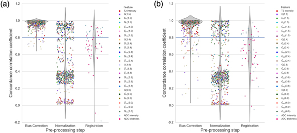
Figure 12. Concordance correlation coefficients between mpMRI features extracted for each pre-processing step and non pre-processed images in (a) healthy tissue and (b) tumor tissue. Each marker represents the concordance correlation for one of the 27 features calculated on the T2w and ADC images. Texture features calculated on the T2w images are denoted by  where G is the Gaussian derivative in direction i at scale s (mm). Values for each of the 31 patients are shown for each feature.
Download figure:
Standard image High-resolution image
Table 6. Features with the lowest mean concordance correlation coefficient (CCC) value across all 31 patients for each pre-processing step.
| Pre-processing step | Feature | Mean CCC (Healthy tissue) | Mean CCC (Tumor tissue) |
|---|---|---|---|
| Bias field correction | T2 intensity | 0.932 | 0.887 |
| G(1.5) | 0.920 | 0.834 | |
| G(2.4) | 0.913 | 0.812 | |
| G(3.8) | 0.902 | 0.783 | |
| G(6.0) | 0.889 | 0.741 | |
| Normalization | T2 intensity | 0.252 | 0.167 |
| G(1.5) | 0.232 | 0.131 | |
| G(2.4) | 0.221 | 0.119 | |
| G(3.8) | 0.206 | 0.107 | |
| G(6.0) | 0.187 | 0.092 | |
| Registration | ADC intensity | 0.763 | 0.661 |
| ADC blobness | 0.664 | 0.598 |
4. Discussion
Results presented in this paper demonstrate that the application of a standardized pre-processing pipeline can improve the capacity of mpMRI to characterize PCa. Each step in the pipeline has the potential to mitigate the effect of artifacts and intensity variability across the dataset, but the greatest improvement in tumor localization using mpMRI was achieved by a combination of multiple pre-processing steps.
The application of PABIC bias field correction to T2w images led to an improvement in tumor localization compared to uncorrected images. A comparison of the performance of PABIC with N4, however, found that the results of the individual metrics (CoV, entropy, and CJV) differed from that of the application-specific task of tumor localization, as measured by the AUC. This is consistent with results presented by Viswanath et al (2011). The authors examined the impact of three bias field correction algorithms (N3 (Sled et al 1998), PABIC, and low-pass filtering (LPF) (Cohen et al 2000)) on the classification of PCa in T2w images. In their study, PABIC was found to minimize CoV and entropy compared with uncorrected images but failed to improve PCa classification. N3, on the other hand, was less successful in reducing CoV and entropy but was comparable to LPF in increasing PCa characterization. A possible explanation for the discrepancy between individual metric results and the outcome of an application-specific task is that the metrics are only indirect measures of performance. This is due to the fact that neither the bias field nor the true intensity spatial distribution is known. Retrospective methods, such as N4 and PABIC, rely almost exclusively on the information contained in the image. While such methods are often easier to implement than prospective ones, validation of the resultant bias field correction can be difficult.
Multiple metrics have thus been used to evaluate the quality of retrospective bias field correction, with measures of intensity variability being some of the most frequently used. CoV lends itself well to the assessment of intensity inhomogeneity because it is invariant to the multiplicative uniform intensity transformation that could be introduced by bias field correction. This metric is limited, though, to use for a single tissue class. Since the intensity values of the PZ are typically hyperintense compared to those of the rest of the prostate gland, the CJV may be a more appropriate measure as it computes the overlap of two tissue classes. This is supported by the fact that CJV was reduced for PABIC compared to N4, which is consistent with the performance of PABIC according to tumor localization. Entropy is an information theoretic measure that offers an alternative means for evaluating intensity variability. It was reduced for both N4 and PABIC but, like CoV, was also found to differ from the results of tumor localization. While each of these three metrics should decrease in value after bias field correction, none of them provides any information as to how much intensity inhomogeneity may remain after bias field correction has been performed. Alternative means of validation have also been proposed, including a comparison of true and estimated bias fields and subsequent segmentation performance. Since a true bias field is typically only available for simulated images and an evaluation of segmentation performance requires ground truth segmentations, which are themselves difficult to obtain due to the intra- and inter-observer variability associated with manual delineation, neither of these methods provides a more definitive measure of bias field correction performance.
Histogram matching normalization was applied to the bias field-corrected T2w images to further improve the accuracy of tumor localization. This result agrees with previous work on bias field correction and normalization in the classification of PCa (Madabhushi and Udupa 2005) since normalization has been shown to have a notable impact on features extracted from T2w images due to the way in which it affects the image information content. Moreover, it is not surprising that the tumor localization model performed better after normalization as it was originally trained using T2w images normalized to the median value in the PZ. The performance of the three normalization methods also differed according to the method of evaluation. Histogram matching yielded a decrease in terms of the CoV and resulted in an increase in the accuracy of tumor localization. Basic normalization, however, led to equally successful tumor localization despite its inability to reduce the CoV. These results are unsurprising because normalization, like bias field correction, is also difficult to validate due to the inherent lack of tissue-specific intensity values of MRI. Alternative metrics have also been proposed to assess normalization, but all are indirect metrics, each with its benefits and limitations. The standard deviation of the normalized mean intensity, for example, has been proposed as an alternative to the CoV in which the mean intensity value within a given tissue is normalized by the range of image intensities (Nyú and Udupa 1999). Even though this metric may be more robust, it must be calculated separately for each acquisition, which may not be the ideal approach for studies that include multiple datasets.
Multi-modal deformable registration of the ADC images to the T2w images did not ultimately improve tumor localization. This can be attributed to the presence of a failed registration result for one or more patients, depending on the registration method used. Given the wide variety of issues that must be overcome in order to achieve an accurate deformable registration, it is difficult to find a single method or set of parameters that will perform well for each patient. The aim of this study was to compare the performance of all three registration methods using the same widely-used algorithm and set of parameters. It is possible, however, that an alternative and better performing algorithm might yield more consistent results across the entire dataset. As this analysis was only meant to be a preliminary exploration of pre-processing performance, a more comprehensive investigation of adequate deformable registration will be a focus of future research.
As with bias field correction and normalization, the individual metrics of registration quality are limited in their ability to provide an accurate picture of the results (see figure S4 in supplementary materials). This is particularly true for non-rigid registration and has been well-documented (Rohlfing 2012). Tissue overlap measures, such as DSC, are only capable of assessing the alignment of the image periphery. They do not evaluate the degree of deformation within the image. There is no single correct value for the Jacobian determinant, but this metric does provide an indication of the nature of the deformation itself. In the case of NiftyReg, for example, the Jacobian determinant value for some of the patients was negative, which indicates that there is inappropriate folding in the deformation. Thus, even though the mean TRE was smallest for NiftyReg, those registrations might not necessarily be optimal. Moreover, the larger values of the mean Jacobian determinant ranges for NiftyReg and ANTs place each of these methods outside of the acceptable range and indicate that the degree of deformation is far too great for some of the registrations. In general, elastix produced the highest quality registrations with the exception of a single patient, which resulted in a poor value for the mean TRE, as well as suboptimal tumor localization in terms of the AUC.
The accuracy of tumor localization was typically greater for those lesions located in the PZ compared with those in the TZ. This is consistent with previous studies that have employed quantitative techniques for the classification of PCa (Lemaître et al 2015), as well as the qualitative assessment of tumor localization using PI-RADS, for which the delineation of tumors within the TZ is traditionally more difficult (Schimmöller et al 2014). The greatest improvement in tumor localization was achieved through the application of multiple pre-processing steps. This is particularly notable in light of the fact that pre-processing itself has been known to introduce additional intensity variation into the imaging data. While previous work has demonstrated the impact of individual pre-processing steps on tumor localization (Viswanath et al 2011, Isaksson et al 2020, Scalco et al 2020), the effect of multiple pre-processing steps on mpMRI of the prostate has yet to be carried out to the best of our knowledge. We show here that by combining multiple, systematically determined pre-processing elements, the accuracy of tumor localization can be increased while simultaneously reducing the impact of intensity variation that may already be present or even newly introduced. Moreover, parameter choice has also been shown to affect pre-processing performance (Boyes et al 2008, Uwano et al 2014, Zöllner et al 2020). As such, this study also emphasizes the importance of optimizing the parameter values of each pre-processing step and its effect on tumor localization performance.
Our assessment of the impact of pre-processing on the features extracted from the T2w and ADC images revealed that the feature values do, in fact, differ with each pre-processing step. This is consistent with previous work that has evaluated the effect of pre-processing on radiomics in prostate mpMRI (Schwier et al 2019). Such results are expected since non pre-processed images are assumed to have some degree of error in the intensity values due to the presence of various image artifacts. Depending on the severity of these artifacts, the pre-processed images will be more or less correlated with the non pre-processed images. If, for example, the mpMRI acquisitions are performed with the use of an endorectal coil, those images would likely require a greater degree of bias field correction and deformable registration and would thus result in pre-processed images that are less correlated with the non pre-processed images. It should be noted, though, that a decrease in the correlation between non pre-processed and pre-processed images is not a sufficient measure of pre-processing performance as there is no formal criteria for how different the pre-processed images should be. It is important, then, to ensure that each pre-processing step is performed appropriately, with improved tumor localization accuracy as the ultimate aim. To this end, we stress the importance of optimizing each pre-processing step and assessing the performance with an application-specific metric.
We chose to focus on some of the most commonly used pre-processing steps for this study, though these are by no means the only ones. Noise filtering, for example, has also been shown to aid in the classification of PCa (Palumbo et al 2011). Moreover, the majority of the pre-processing was applied to the T2w images because these were the greatest source of mpMRI features used to generate the tumor probability maps. It has been shown, however, that normalization of ADC images can also improve diagnostic accuracy (Taha Ali et al 2018). It is thus possible that the incorporation of additional pre-processing steps could improve the tumor localization results even further. Future work will consist of the assessment of pre-processing steps that might be applied to DW images, including bias field correction prior to multi-modal registration, normalization, and denoising. Moreover, motion correction and normalization of the DCE images will also be considered. Since the Ktrans images underwent ROI normalization in order to be consistent with the mpMRI data used to train the tumor localization model, exploring alternative methods of Ktrans normalization would be a logical extension of the current analysis. The resultant pre-processing pipeline and tumor localization model will then be applied to multi-site prostate mpMRI for which image variability is more pronounced and standardization is increasingly important. Additionally, given the variability of imaging data from one site to another and the corresponding differences in pre-processing requirements for each dataset, future work will also include an evaluation of the trade-off between pre-processing parameter optimization and improvement in tumor localization accuracy.
While the optimized pre-processing pipeline developed in this study was found to improve the accuracy of tumor localization, there is no guarantee that this particular optimization would hold for mpMRI data acquired from other institutions. In fact, it is likely that some degree of optimization would still be required before implementing this pipeline on an alternative dataset in order to obtain comparable results. Further validation of the proposed method on external datasets will be required in order to determine how well this approach can be generalized to imaging data acquired under different conditions and on different scanners. By tailoring the pre-processing steps to a given mpMRI dataset, however, we were able to improve the performance of the tumor localization model without the need for any retraining. In this way, the tumor localization model may be robust to use on multiple different datasets in which retraining with the required ground truth prostatectomy specimens is impractical or even impossible.
5. Conclusion
We demonstrate that the application of a comprehensive pre-processing pipeline can improve the ability of mpMRI to characterize prostate tumors with a model-based approach. A systematic evaluation of several data preparation and pre-processing steps found that different methods give variable results and that assessment with individual metrics may not always coincide with the performance of the ultimate aim of tumor localization. These results highlight not only the effect that a combination of multiple pre-processing steps may have on the characterization of PCa, but also on the need for further standardization and validation of quantitative mpMRI analyses of the prostate.
Acknowledgments
This research was supported by the Réseau en Bio-Imagerie du Quebec (RBIQ 35450).
Supplementary data (5.3 MB DOCX)