
Abstract
We present a mechano-chemical model that couples corrosion, mechanical response, and fracture. The model is used to understand the failure of Cu wires on Al pads in microelectronic packages using a multi-phase field approach. Under high humidity environments, the Cu-rich intermetallic compounds (IMC), Cu9Al4, formed at the interface between Cu and Al, undergo a corrosion degradation process. The IMC expands while undergoing corrosion, inducing stresses that nucleate and propagate cracks along the interface between the Cu-rich IMC and Cu. Furthermore, the volumetric expansion of the IMC may cause damage to the passivation layer and enhance the nucleation of new corrosion pits. We show that the presence of a crack accelerates the corrosion process. The model developed here can be extended to other systems and applications.
Export citation and abstract BibTeX RIS

Original content from this work may be used under the terms of the Creative Commons Attribution 4.0 license. Any further distribution of this work must maintain attribution to the author(s) and the title of the work, journal citation and DOI.
1. Introduction
Corrosion is an electrochemical reaction between a metal and its environment that leads to the degradation of the material. In particular, fracture induced by corrosion leads to failure in a wide variety of applications, including aerospace [1], biomedical [2], structures [3, 4], batteries [5], and microelectronics [6–8]. We present a model that couples corrosion with volumetric expansion creating stresses that nucleate and propagate cracks. The model is applied to understand failure in Cu wire-bonded integrated circuits.
The electrical connection between a die and the package is made using wire bonds. The aluminum pad is connected to gold or copper wires. Due to lower costs, and lower thermal and electrical resistivity copper wires are most widely used. One of the challenges in the Cu/Al bonding is the higher hardness and susceptibility to oxidation of the intermetallic compound (IMC) phases. Experimental work in Cu/Al systems shows that corrosion occurs in the phase with the highest concentration of Cu due to humidity and high temperature. As a consequence of corrosion the IMC volume expands and cracks nucleate and propagate reducing the reliability of the bond.
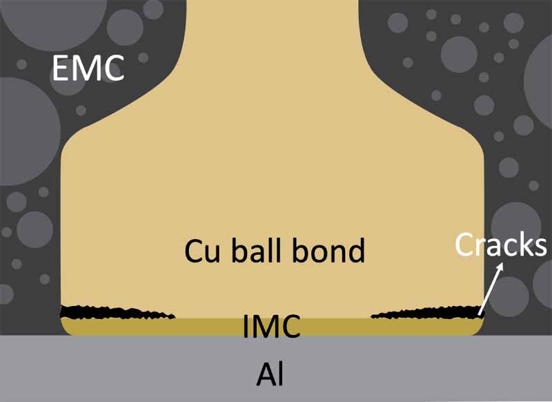
The IMCs identified at Cu/Al interfaces are CuAl2, CuAl, and Cu9Al4. Even though Al is the most electrochemically active, Al passivation oxides prevent the corrosion of Al and Al-rich IMCs. Passivation oxide pitting is observed primarily in the Cu9Al4 and therefore, this is the first phase to be corroded [9–13]. Boettcher et al [13] observed the resulting oxidized interface which is highly susceptible to fracture and therefore, the ultimate reason for failure. A schematic of a Cu ball bound to an Al pad with IMCs, and cracks, enclosed in an epoxy mold compound is shown in figure 1. The diameter of the Cu ball is approximately in the range of 40–100 μm [10, 14].

Figure 1. Schematic of crack failure in a Cu ball bump on an Al pad showing the IMC, the epoxy mold compound (EMC), and cracks.
Download figure:
Standard image High-resolution imageThe experiments by Rongen et al [9] show simultaneous corrosion and crack evolution in Cu/Al bonds with temperatures from 110 °C to 225 °C and relative humidity (RH) 75%–95%. The corrosion front and cracks advance inwards from the outer surface to the center. The rate of growth increases with temperature and RH reaching around 20 μm in length at rates of up to 0.06 μm h−1.
Lall et al [15] simulate the corrosion of Cu/Al wire bonds solving the transport equation for chlorine. One of the difficulties of the approach is the changing boundary condition as the corrosion front advances. Other numerical efforts to simulate corrosion in different materials systems overcome this limitation by using a sharp interphase method [2, 16] and phase field approaches [2, 17].
Mai et al [17] developed a phase field approach based on the Kim-Kim-Suzuki [18] (KKS) model to track the corrosion front in stainless steel in an electrolyte solution. The model was later enhanced to incorporate the effect of material degradation, through a reduction of the stress intensity factor, to simulate the effect of corrosion on fracture [19]. Similarly, Chen and Bobaru [4] simulate the corrosion front along with the nucleation of cracks that appear as a result of bond rupture during chemical reactions in Mg alloys. The authors use the peridynamics model to include the formation of cracks. Kovacevic et al [2] use a phase field model to simulate the corrosion of Mg alloy in body fluids. Their framework captures pitting corrosion and accounts for the synergistic effect of aggressive environments and mechanical loading in accelerating corrosion kinetics. To account for that, the corrosion kinetics is modified by a factor that depends on local stress and strain distributions. Toongoenthong and Maekawa [20] use a non-linear mechanics finite element model to simulate the corrosive crack inside reinforced concrete due to the volumetric expansion of the corrosive product of steel. The corroded region is predefined in the geometry with the volumetric expansion strain obtained from experiential data.
In this study, we present a multi-phase field method that tracks the evolution of corrosion using a KKS model. Simultaneously, this field is used to calculate the volumetric expansion of the oxidized material resulting in stresses that nucleate and propagate cracks that in turn affect the diffusion and accelerate corrosion. We use this model to study the corrosion and subsequent cracks that appear in the IMC phases of Cu–Al wire bonds. The paper is organized as follows. In section 2 we present the corrosion and mechanical models. In section 3, we present axisymmetric and 3D simulations in Cu–Al systems with the summary in section 4.
2. Model
Experiments by Osenbach et al [11] show selective oxidation of the Al in Cu9Al4 that results in the formation of a two-phase microstructure composed of γ-Al2O3 with embedded crystalline Cu metal particles. We use a simplified model for the corrosion reaction following [11]:


It is important to note that different reaction processes are described in other references [9]. In both references the corroded region is  , which is the concentration that we are going to track without considering intermediate steps. The volumetric expansion of the corroded phase (γAl2O3) induces stresses that cause cracks to nucleate and propagate at the interface between Cu9Al4 /Cu and Cu.
In the following sections, we present a multi-phase field model to simulate the evolution of corrosion and track the growth of cracks. The chemical evolution is coupled to the mechanical response through the volumetric expansion of the corroded phase. The elasto-plastic response of the components of the system is used to calculate stresses that drive the nucleation of cracks that appear at the Cu9Al4/Cu interface.
2.1. Corrosion
Consider a metal immersed in a solution, as shown in figure 2. The metal surface has a passivation layer that makes it resistant to corrosion. However, in the presence of a pit in the passivation layer, the corrosion can advance into the metal following the equilibrium between the dissolved metal atoms flux and the velocity of the pit boundary [17] as


Figure 2. A schematic of pit corrosion in a metal. The field,  , tracks the concentration of metal atoms.
Download figure:
Standard image High-resolution imagewhere  tracks the concentration of metal atoms, cs is the concentration of atoms in the intact metal,
  is a diffusion coefficient,
  is the velocity of the pit boundary, and
n
is the normal to the surface.
is the velocity of the pit boundary, and
n
is the normal to the surface.
Initially, the process is activation controlled, and the pit velocity follows Tafel's equation [17]. When the concentration,  , reaches the saturation concentration, csat, the process is controlled by diffusion, and the pit boundary normal velocity is given by

The solution of equations (3) and (4), known as the Stefan problem [21–24], requires imposing a boundary condition  in the moving boundary
  . Here we use a phase field approach to follow the interface between the intact and corroded metal.
Following Mai et al [17] a phase field variable  is used to track the corroded material, with
  in the corroded or aqueous region and
  in the intact metal. To follow the concentration fraction of metal atoms, we define the concentration normalized by

The total free energy of the system is given by [18, 25]

The first term in the integral in equation (6) is the local free energy density, the second is the interface energy, and the third is a double well potential. In equation (6)  and w are coefficients that control the thickness of the interface and are defined in terms of the interface energy density
  and the interface thickness
  by [18]


Following the KKS model [18] the concentration is interpolated by the concentration of the two phases

where  is the concentration of metal atoms in the intact metal and
  is the concentration in the corroded material, and
  is an interpolation function. Similarly, the local free energy density is written as an interpolation between the free energies densities of the two phases following

The free energy density functions for each phase can be approximated by a parabolic function with the minimum energies at the intact metal concentration  , and boundary condition
  .
.


where  is a coefficient
  , and
, and  are the normalized equilibrium concentrations following the definition in equation (5). Finally, the free energy densities must satisfy the equilibrium of chemical potential

The evolution of the phase fields follows the Allen–Cahn equation for the non-conserved field  and the Cahn–Hilliard equation for the conserved variable
  [18]
[18]


where  is a kinetic parameter that controls the velocity of the interface, and
  is a diffusion coefficient. The functional derivatives
  and
and  in equations (14) and (15) are derived in Kim et al [18].
The first chemical reaction in equation (1) is used to calculate csat which is determined by the metal atom concentration in  [2, 17]. Similarly, cs is the metal atom concentration of
  . Following Scheiner and Hellmich [26] we write the mass density of
  as:
as:

where  is the specific concentration of the species i,
  is the atomic % (note that it is equivalent to the mole fraction defined in reference [26]),
  is the molar mass, and
  .
.
With  = 6.85 g cm−3 for
  and using the values in table 1 we obtain
  and
and  = 0.131 mol cm−3. Repeating the procedure for AlCl3 we obtain
  g mol−1. Using
  = 2.48 g cm−3 for AlCl3, we obtain
  = 0.075 mol cm−3 and using equation (5),
  .
.
Table 1. At% and molar mass Cu9Al4 and AlCl3.
| # at | at% 
| Molar mass (g mol−1) Mi | ||
|---|---|---|---|---|
| Cu9Al4 | Cu | 9 | 9/13 | 63.5 |
| Al | 4 | 4/13 | 26.9 | |
| AlCl3 | Cl | 3 | 3/4 | 35.5 |
| Al | 1 | 1/4 | 26.9 |
2.2. Mechanical response
The mechanical responses of Cu and Al include plasticity, a fracture model is used in the IMC domain, and we incorporate the volumetric expansion of the corroded material [27]. The strain is decomposed into the elastic,  and plastic,
  parts
parts

The plastic strain follows an isotropic flow rule

where the components of the deviatoric stress are  ,
,  is the von Misses stress (using Einstein's notation), and
  is the rate at which plastic strain occurs. We assume perfect plasticity with a flow rule [28]

where  is the yield stress. The irreversibility of the plastic deformation is obtained with the Kuhn/Tucker conditions:

These conditions allow plastic deformation only when  .
.
To track the evolution of cracks we use a phase field damage model [29–31] in which the field d(x) indicates undamaged material when d = 0 and damage when d = 1. The strain energy of the system is written as

The first term on the right-hand side of equation (21) is the fracture energy and the second is the integral of elastic strain energy density:

where  is the part of the strain energy density that is degraded with damage and
  is not affected by damage and are defined by


 and
and  are Young's modulus and Poisson's ratio, 〈x〉 = x if
  , and 〈x〉 = 0 otherwise, and
  . Note that when d = 0, we recover the classical strain energy density as
  . The fracture energy follows Griffith's criterion for brittle materials over the crack surface Γ [32]

where  is the fracture surface energy density. The integral over the crack surface,
  can be replaced by an integral over the volume using a diffuse delta function in terms of the damage field [33–35]

where  is the effective crack width [29–31, 33].
The evolution of the damage follows as

The rate of energy dissipation due to cracks should be positive,  , this leads to
  i.e. the cracks can only grow with time. The mechanical response relaxes faster than the corrosion evolution, and therefore, we consider the steady state form of the conservation of linear momentum:

where  is the Cauchy stress tensor defined by

2.3. Mechano-chemical coupling
The Pilling–Bedworth (P–B) ratio [36, 37] is the ratio of the volume of the elementary cell of metal oxide,  , to the unit volume of the metal,
  , and it can be used to estimate the change in volume due corrosion [38]. This ratio is defined as

where n is the number of metal atoms in the oxide molecule. Note that equation (30) considers that the metal is a single component. Therefore, we will use here that  cm3 mol−1 given the at% of 1 atom of Al in Cu9Al4. Using n = 2.67 and
  , see table 2, we obtain PBR = 1.8, which represents an 80% volumetric expansion of the γAl2O3 due to corrosion. We assume that only Al in the Cu9Al4 phase is corroded as Cu precipitation is observed in the experiments [11]. Therefore, the volumetric expansion is proportional to the at% of Al in Cu9Al4, see table 1, which results in
Table 2. Mass density, molar mass, and volume of Cu9Al4 and  -Al2O3.
Mass density  (g cm−3) (g cm−3) | Molar mass Mi (g mol−1) | Molar volume Vi (cm3 mol−1) | |
|---|---|---|---|
| Cu9Al4 | 6.85 | 679.84 | 99.12 |
 -Al2O3 (Al2.67O4) -Al2O3 (Al2.67O4) | 3.67 | 136.04 | 37.07 |
The field  used to indicate the corrosion in section 3.1 is used to track the volumetric expansion of the
  Al2O3,

where  ,
,  corresponds intact material, and
  is the volumetric expansion coefficient.
2.4. Corrosion calibration
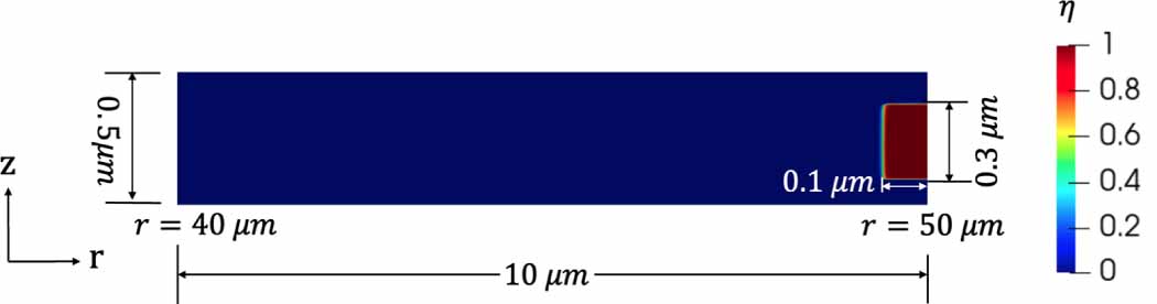
The KKS model presented in section 2.1 is implemented in the finite element solver MOOSE [39] to solve equations (14) and (15) using cylindrical coordinates with an element size 40 nm. A 50 μm radius Cu ball bond is considered in these simulations to compare with experimental results [9].
The mechanical part is not included in this section and we track only the evolution of the corrosion fields  and
and  (x,t) in the Cu9Al4 region. Figure 3 shows the dimensions and initial conditions.

Figure 3. Geometry and initial conditions used to calibrate the corrosion model.
Download figure:
Standard image High-resolution imageThe right boundary (outer surface) has a pit opening represented by a region with  and
and  . Given that the initial corroded region will advance less than 10 μm from the outer surface during the simulation time we only simulate the region 40 μm ⩽ r ⩽ 50 μm Therefore, the region r ⩽40 μm contains intact material and we impose no flux of
  and
and  in this boundary as well as the top and bottom boundaries.
The interface energy density,  , is reported in literature for metal corrosion is in the range of 0.1–10 J m−2 [2, 17, 40]. Therefore, we choose the interface energy density between the corroded material and the uncorroded material as
  J m−2 and an interface thickness
  300 nm, which is seven times the element size. These values are used to calculate
  and
and  in table 3. The experimental data in [9] is used to calibrate the other parameters in the simulation.
Table 3. Parameters used in the corrosion model.
 ( ( ) ) |

|
 ( ( ) ) |

|
 ( ( ) ) |

|

| 0.57 |

|

|
 ( ( ) ) |

|
 ( ( ) ) | 2 |
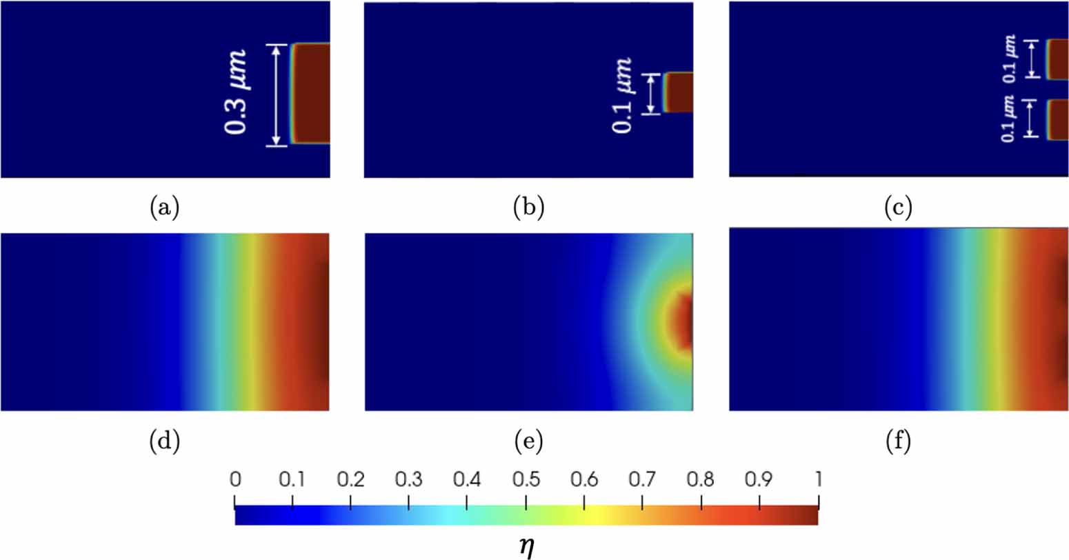
Geometries featuring different pit sizes and varying numbers of pits are shown in figures 4(a)–(c). The boundary profiles at t = 0.5 h are shown in figures 4(d)–(f) and the evolution of the corrosion boundary location S(t) is plotted in figure 5. S(t) is the location of  and it is measured from the outer surface. S(t) is plotted as a function of the square root of time because the 1D analytical solution follows
  . Due to the zero flux boundary conditions, once the corrosion reaches the top and bottom surfaces its profile is flat and the velocities are identical for the three cases following the form
  , see figure 5. Since there is no difference in the corroded material profile after 1 h, single 0.3 μm and 0.5 μm pits are chosen for the following simulations.
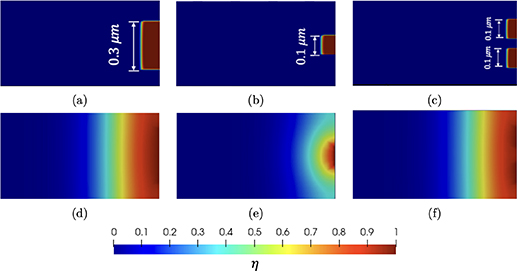
Figure 4. Geometries with (a) one 0.3 μm pit (b) one 0.1 μm pit (c) two 0.1 μm pits. Contour plot of  at t = 0.5 h for (d) one 0.3 μm pit (e) one 0.1 μm pit (f) two 0.1 μm pits.
Download figure:
Standard image High-resolution image
Figure 5. Comparison of the corrosion boundary location as a function of time for different pit configurations.
Download figure:
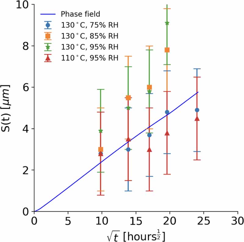
Standard image High-resolution imageRongen et al [9] utilized scanning electron microscopy to measure the corrosion product and the intact metal radii in a Cu ball with a diameter of approximately 50 µm. The experiments were conducted with temperatures 110 °C and 130 °C, with RH levels of 75%, 85%, and 95%. Figure 6 shows the position of the corrosion pit as a function of time from Rongen et al [9] and our simulations. Lower temperatures reduce diffusivity, resulting in slower corrosion velocities. The parameters used in the simulation to obtain similar corrosion pit velocities are listed in table 3. It is important to notice the large uncertainty in the experiments, therefore, the mobility parameters in table 3 need to be considered an approximation.

Figure 6. Corrosion boundary location S(t) obtained from the phase field simulations and experimental data from [9].
Download figure:
Standard image High-resolution image3. Results
The corrosion and mechanical models described in section 3 are implemented and solved using the finite element solver MOOSE [39] with the geometries in figures 7 and 8. Figure 7 is axisymmetric and the simulations are solved with cylindrical coordinates. A pit opening is located at  in the Cu9Al4 region and the geometry includes only the outer region of the Cu ball from
  to
to  . The corrosion pits have a fixed boundary condition
  and
and  . The other boundaries are assigned zero flux for
  and
and  . The element size in the Cu, Al, and Cu9Al4 is 40 nm, while the elements close to the Cu9Al4/Cu interface are 15 nm. The interface thickness and crack width parameter are chosen to be
  = 300 nm and
  75 nm.

Figure 7. Axisymmetric geometry used in the simulations.
Download figure:
Standard image High-resolution image
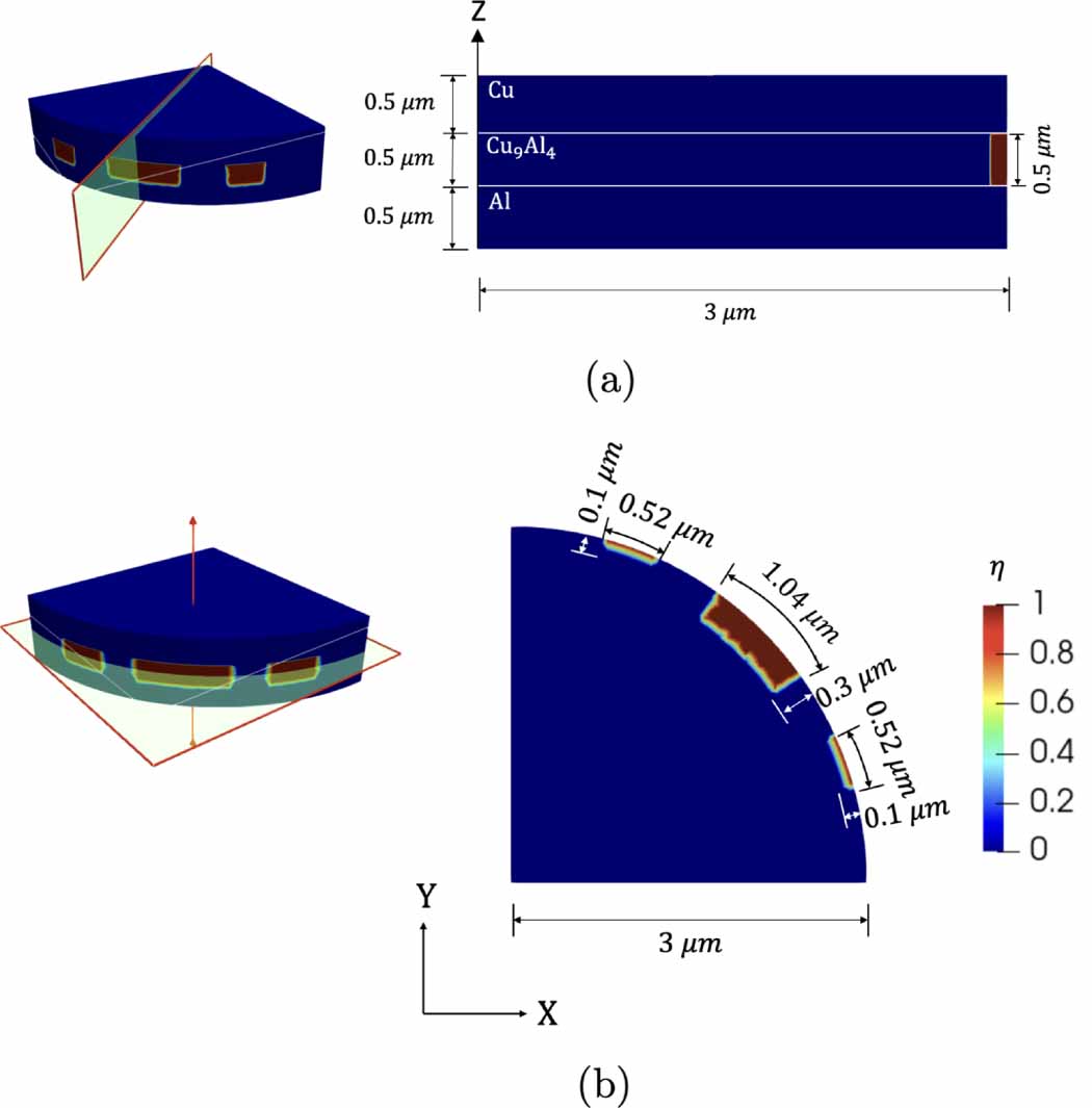
Figure 8. 3D geometry (a) shows the vertical cross-section and (b) shows the horizontal cross-section.
Download figure:
Standard image High-resolution imageIn the 3D figure 8, the same Cu/Cu9Al4/Al sandwich structure is adopted. The domain is a quarter of a disk with a radius of 3 μm and 3 pits in the Cu9Al4 layer. Periodic boundary conditions are imposed on the sides of the disk for  and
and  . The element size in the Cu, Al, and Cu9Al4 is 130 nm, and the elements close to the Cu9Al4/Cu interface are 25 nm. The corrosion interface thickness and crack width parameter are chosen to be
  = 650 nm and
  140 nm. Figure 9 shows the displacement boundary conditions for both geometries. The parameters used in the simulations are listed in tables 3 and 4.

Figure 9. Displacement boundary conditions used in the (a) axisymmetric and (b) 3D geometries.
Download figure:
Standard image High-resolution imageTable 4. Material properties used in the simulations, * indicates an estimated value.
| Cu | Al | Cu9Al4/Cu | Cu9Al4 |
 Al2O3 Al2O3
| |
|---|---|---|---|---|---|

| 130 [46] | 70 [46] | 187 [42] | 187 [42] | 372 [46] |

| 0.34 [46] | 0.35 [46] | 0.3 [42] | 0.3 [42] | 0.25 [46] |

| 200 [46] | 100 [46] | — | — | — |
| Gc (J m−2) | 707 | — | 5* | 25 | 35 |

| 10.2 [44, 45] | — | — | 2.3 [41, 42] | 3.7 [43] |
As the corrosion advances and Cu9Al4 transforms to corroded material, the Young's modulus and fracture energy are interpolated as a function of the phase variable  :
:


where  and
and  are Young's modulus and fracture energy of the corroded material. The corroded region is identified by
  consists of
  and Cu precipitates [11]. The Young's modulus
  in this region is the average by area fraction from figure 4 in reference 11 as
  0.7 ECu + 0.3
  = 204 GPa.
The fracture surface energy is related to the fracture toughness  as:
as:

For Cu9Al4 a range of values  is reported from 0.7
  to 3.0
  [41, 42], for
  Al2O3
Al2O3
 [43], for Cu from 8
  to 14
to 14  [44, 45]. The fracture surface energies Gc
in table 4 are calculated from equation (33). To include that the Cu9Al4/Cu interface is weaker, a reduced fracture surface energy is used in a 100 nm thick layer to represent this region. Similarly to the Young modulus, the surface energy of the corroded material is approximated as
[44, 45]. The fracture surface energies Gc
in table 4 are calculated from equation (33). To include that the Cu9Al4/Cu interface is weaker, a reduced fracture surface energy is used in a 100 nm thick layer to represent this region. Similarly to the Young modulus, the surface energy of the corroded material is approximated as 
 .
.
3.1. Axisymmetric geometry
Figure 10 shows the evolution of corrosion field  , figure 11 shows the volumetric stress
  , and figure 12 shows the shear component in the stress tensor,
  . The surrounding material inhibits the volumetric expansion of the corroded material, resulting in high compressive stress, see figure 11. Large shear stresses in the crack tip and in the Cu9Al4/Al are shown in figure 12. The shear stress in the Cu9Al4/Cu interface drive the growth of the crack as the corroded material expands.

Figure 10. Axisymmetric simulations, corrosion field contour plots with cracks marked in white for d > 0.9 at (a) 4 h, (b) 70 h, and (c) 300 h.
Download figure:
Standard image High-resolution image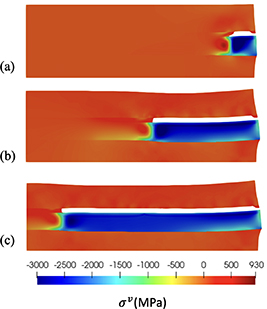
Figure 11. Axisymmetric simulations, volumetric stress contour plots with cracks marked in white for d > 0.9 at (a) 4 h, (b) 70 h, and (c) 300 h.
Download figure:
Standard image High-resolution image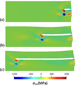
Figure 12. Axisymmetric simulations, shear stress contour plots with cracks marked in white for d > 0.9 at (a) 4 h, (b) 70 h, and (c) 300 h.
Download figure:
Standard image High-resolution image3.2. 3D geometry
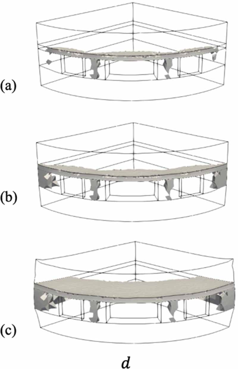
The evolution of the corrosion field in the 3D geometry is shown in figure 13. Corrosion starts at the three pits and the corroded regions merge forming a smooth front. The differences in time scales between the axisymmetric and 3D simulations are due to the different radii used in the geometries, 50 μm in the axisymmetric versus 3 μm in the 3D simulations. The time evolution of the position of the corrosion boundary is inversely proportional to the radius of the outer surface [47] and therefore, the rate of growth is higher in the 3D simulations.

Figure 13. Propagation of corrosion in the 3D geometry at (a) 1 h, (b) 2.8 h, and (c) 15.8 h. Corrosion field is shown only for  .
.
Download figure:
Standard image High-resolution imageFigure 14 shows the damage field in the 3D geometry. The volumetric expansion due to the corrosion of the Cu9Al4 layer causes localized shear stresses between the pits in the surface of the Cu ball during the early stages (<1 h), see figure 15. Therefore, more pits could be nucleated in these regions and accelerate the corrosion process.
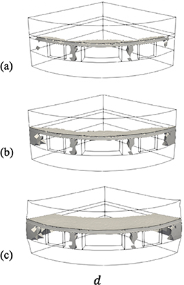
Figure 14. Damage propagation in the 3D geometry at (a) 1 h, (b) 2.8 h, and (c) 15.8 h. Damage in grey for  .
.
Download figure:
Standard image High-resolution image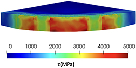
Figure 15. Von Mises stress at 1 h, only the Cu9Al4 layers is shown.
Download figure:
Standard image High-resolution image3.3. Damage-induced corrosion acceleration
Damage to the outer surface of the Cu ball in the Cu9Al4/Cu interface could induce the formation of new pits and therefore, accelerates the corrosion through faster diffusion of Cl− . To take into account the coupling between damage and corrosion, we increase the diffusivity in the damaged regions with the following relationship:

where  is a switch function that identifies the crack region, i.e.
  if
if  , and
, and  otherwise, and
  is a parameter. Note that in the regions without damage we recover the value of
  listed in table 3. Figure 16 shows the corrosion boundary profile for K = 0, 30, 50, and 100 at 12 h. When K is not zero the mobility is increased in the crack region and the corrosion advances at a faster rate in the Cu9Al4/Cu interface forming a slanted profile. Due to this profile shape, a tensile stress appears in the Cu9Al4/Al in front of the corrosion boundary, see figure 17. That leads to the damage in the Cu9Al4/Al interface shown in figure 18.
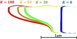
Figure 16. Corrosion boundary profile for K = 0, 30, 50, and 100 at 12 h.
Download figure:
Standard image High-resolution image
Figure 17. Zoom of the volumetric stress contour plots with cracks marked in white for d > 0.9 at 12 h for K = 100.
Download figure:
Standard image High-resolution image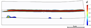
Figure 18. Damage field contour plots at 44 h for K = 100. Damage is only shown for d > 0.5.
Download figure:
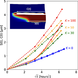
Standard image High-resolution imageFigure 19 shows the position of the crack tip, C(t), and the corrosion boundary, S(t), measured from the Cu ball surface. As expected, enhancing the diffusion coefficient in the crack increases the rate of growth of the corroded region which in turn accelerates the damage.
Figure 19. Comparison of the corrosion boundary and crack locations for different K values.
Download figure:
Standard image High-resolution image
4. Summary
A mechano-chemical model that couples corrosion, mechanical response, and fracture was developed. The model includes a KKS approach to solve the corrosion evolution, the stresses that arise due to volumetric expansion of the corroded material, and a phase field damage model to track the evolution of cracks. The model can be extended to study other systems. Here, the model was used to investigate the failure of Cu/Al wire bonding commonly employed in microelectronic packaging.
Corrosion affects the Cu-rich phase of the IMC layer in Cu/Al bonding. This occurs because the passivation layer is weaker in the Cu9Al4 phase and pits form there. The corroded material consists of  and Cu precipitates. This transformation renders a volumetric expansion of the corroded material of approximately 24% calculated from the P–B ratio between the Al in Cu9Al4 and
  Al2O3. The stresses resulting from this volumetric expansion drive the formation of cracks at the Cu9Al4/Cu interface leading to failure in agreement with experimental results [9, 13].
Damage to the outer surface of the Cu ball in the Cu9Al4/Cu interface may induce the formation of new pits. To consider this, the diffusivity is increased in the damaged regions following equation (34). As expected, the corrosion rate and the crack tip velocities grow. More importantly, this changes the profile of the corroded region from a planar, see figure 10, to oblique, see figure 16. Due to this, tensile stresses appear close to the Cu9Al4/Al interface developing damage.
While 2D and axisymmetric geometries can estimate the corrosion rate, 3D simulations are needed to investigate the effect of pit locations. In the 3D simulations, we observe that the shear stresses developed between pits in the IMC layer due to the volumetric expansion. These shear stresses may induce damage in the passivation layer and nucleate new corrosion pits that will enhance the corrosion process.
Unfortunately, quantitative comparison to experiments is limited due to the lack of data on some key parameters in the model. For example, the saturation concentration of metal atoms in the corroded region controls the rate of corrosion. This value was calculated from the molar mass of AlCl3 as csat = 0.075 mol cm−3. However, this is an approximation and the atomic concentration in the surface needs to be measured experimentally to improve our predictions. Other parameters, such as interface energies and mobilities have been approximated due to the lack of experimental data.
Acknowledgments
This work was supported by Semiconductor Research Corporation. We would like to thank Professor Muhammad A Alam (Purdue) and M Asaduz Zaman Mamun (Purdue) for insightful discussions.
Data availability statement
The data cannot be made publicly available upon publication because they are not available in a format that is sufficiently accessible or reusable by other researchers. The data that support the findings of this study are available upon reasonable request from the authors.