

Abstract
The present work concerns the modeling of the Payne effect in nonlinear viscoelasticity. This effect is a characteristic property of filled elastomers. Indeed, under cyclic loading of increasing amplitude, a decrease is shown in the storage modulus and a peak in the loss modulus. In this study, the Payne effect is assumed to arise from a change of the material microstructure, i.e. the thixotropy. The so-called intrinsic time or shift time was inferred from solving a differential equation that represents the evolution of a material's microstructure. Then, the physical time is replaced by the shift time in the framework of a recent fractional visco-hyperelastic model, which was linearized in the neighborhood of a static pre-deformation. As a result, we have investigated the effects of static pre-deformation, frequency, and magnitude of dynamic strain on storage and loss moduli in the steady state. Thereafter, the same set of parameters identified from the complex Young's modulus was used to predict the stress in the pre-deformed configuration. Finally, it is demonstrated that the proposed model is reasonably accurate in predicting Payne effect.
Export citation and abstract BibTeX RIS
1. Introduction
Rubber components are widely used as elastic connections in engineering structures to achieve a combination of stiffness and vibration isolation [1]. The best example is the engine mounts in the automotive and aircraft industries. Also, the tire performance is related to the thermal and viscoelastic properties of rubber of tires. Indeed, Ebbot et al [2] have proposed a coupled thermo-mechanical model, in which the stiffness and the loss are functions of the strain, temperature, and loading frequency.
Accordingly, the design of these rubber parts requires considering various complex effects: frequency, pre-load, thixotropy, etc. Much research has been devoted to study all these dependencies, particularly for carbon black-filled rubber (CBR) which usually present complex behaviors [3, 4]. The effects of Mullins and Payne are intrinsic to the behavior of reinforced rubbers (by carbon black or silica). The stress-softening phenomenon or the Mullins effect is characterized by a loss of stiffness during the first cycle of loading [5, 6]. This loss of rigidity will then be common to the following cycles (loading/unloading), that is provided that the applied strain does not go beyond the maximum strain reached in the history of deformation. Several authors have attributed the Mullins effect to bond rupture [7], molecular disentanglement [8], and multiple networks [9, 10]. Phenomenological descriptions of the Mullins effect was proposed in the framework of the continuum damage mechanics [11–14]. The reader may refer to a recent review article by Diani et al [15]. We note that the Mullins effect remains a hurdle in the formulation of hyperelastic models. Indeed, one should remove it experimentally in order to reach a stable material behavior, i.e. the hyperelastic behavior. Consequently, the rubbers are subjected to preloading conditions [16]. Hyperelastic models are usually used to represent the elastic behavior of rubbers undergoing large deformations [17, 18]. The reader may refer to a recent review article by [19]. Rubber-like materials exhibit also strain stiffening effects arising from limiting molecular chains extensibility; the simplest model of this type is due to Gent [20]. This model was used to represent the hyperelastic response of dielectric elastomers [21, 22]. Any bibliography on the subject of modeling rubber-like materials remains incomplete.
Under time-harmonic cyclic loading of increasing amplitude, filled elastomers show a decrease in storage modulus and a peak in loss modulus. This strain amplitude dependence is referred to as the Payne effect [23]. It was also shown that increasing the magnitude of strain for a given frequency will decrease the storage modulus monotonically; while the loss modulus increases reaching a maximum and then decreases. Both the storage and loss moduli decrease with a decrease in frequency for a fixed value of the amplitude of strain. Changes in dynamic moduli of filled elastomers seem to be related to the aggregation of filler particles into clusters and networks [24, 25]. The Payne effect has been a subject of numerous theories [26–30].
For instance, Lion and Kardelky [31] have developed a constitutive approach of finite viscoelasticity to represent the Payne effect in a continuum framework. The constitutive relationship is of integral form, in which the hyperelasticity is modeled by a neo-Hookean model, and the physical time variables are replaced by process-dependent intrinsic times. Then, the integral constitutive equation is transformed using a complicated computation into a differential equation similar to that of the classical Maxwell model of linear viscoelasticity. The differential constitutive model was linearized in order to compute the harmonic complex Young's modulus. Consequently, the loss modulus does not depend on the pre-stretch. This result seems not to be consistent with experimental results [32–37]. Recently, Narayan and Palade [38] have noticed a similarity between the behaviors of thixotropic fluids and filled elastomers. Therefore, the internal microstructure of a material can be characterized by a scalar parameter or second-order tensorial called 'structure parameter' originated from changes of the thixotropy, i.e. on changes of the viscosity [39, 40]. As a result, two approaches have been developed to model the Payne effect [38]. The first was based on a thermodynamic framework involving multiple natural configurations, while the second used the concept of 'structure parameter'. These authors have shown that, their models fall short of capturing the Payne effect apparently due to inappropriate choice of both the Helmholtz potential and rate of dissipation.
In experiments, the dynamic properties of elastomers can be described by the linearized steady-state response, i.e. small sinusoidal vibrations that are superimposed on large static deformation. The static stress is due to pre-strain and determined only by the last state of static deformation; so that; it does not depend on the deformation history. Consequently, the viscoelastic effects depend only on superimposed small vibratory deformations [41, 42]. Classically, viscoelastic models are derived from two approaches, namely integral and internal variables approaches. So, many models have been proposed for large strain viscoelasticity and their numerical implementation in finite elements (FE) [14, 34, 35, 43–58] to mention a few. Furthermore, the response of soft materials and biological tissues can be strain-rate dependent; the Helmholtz free energy function is written in terms of external thermodynamic state variables. As a result, the nominal stress is expressed as the sum of the hyperelastic nominal stress corresponding to the quasi-static equilibrium state, the viscous overstress arising from high strain rate and stress due to long time memory effect [59]. We point out that a detailed review of the various visco-hyperelastic modeling approaches as well as an external-state variable based models have been proposed by [60]. One drawback of the integral models is probably their high number of material parameters, which are necessary to reproduce experiments. In engineering designs, the constitutive models should be simple with few material parameters, which are easy to determine using experimental data of standard testing. We recall that many models have extended the generalized Maxwell (GM) model of the linear viscoelasticity to finite strains. The GM model can capture almost a full frequency range of the experimental data. However, it produces local 'oscillations' [61, 62], and existing literature on this subject does not provide a convincing interpretation of this phenomenon. To overcome this difficulty, the fractional derivative-type models seem to be more attractive because the relaxation functions of elastomeric materials can be predicted with fewer material parameters.
In the present work, we have developed the integral version of the constitutive equation, i.e. equation (24) of Bouzidi et al [63], in which the thixotropy was not accounted for. To model the Payne effect, the so-called intrinsic time or shift time concept was used, which arises from a change of the material microstructure. Additionally, the Mooney–Rivlin hyperelastic model (instead of the neo-Hookean one) was considered to investigate the coupling between material nonlinearity and relaxation. So, the range of large strains, i.e. the order of 100% could be reached. As a result, the constitutive relationship was linearized in order to highlight the effects of pre-strain, the magnitude of dynamic strain, and frequency. Thereby, special attention will be paid to the small harmonic vibrations that are superimposed on a large static deformation; this loading is relevant in many engineering designs.
This paper is organized as follows: in section 2, we briefly summarize the basics of the visco-hyperelastic model already presented and analyzed in previous works. The third section covers the linearization of the proposed model, whereas section 4 is devoted to the computation of the harmonic complex Young's modulus in the pre-deformed configuration. The identification of the material parameters and checking predictions of the model are presented in section 5.
2. Presentation of the model
Let F = ∂x/∂X be the deformation gradient tensor, where X is the position vector of a material particle in the undeformed configuration and x is the corresponding position in the deformed configuration.
The right and left Cauchy–Green strain tensors are denoted by C = FT
F and B = FFT
, respectively. The principal invariants of C (or B) are given by  ,
,  ,
,  [17].
[17]. and
and  are the Green–Lagrange strain tensor and Piola strain tensor, respectively, and I is the identity tensor.
Combining both the one-dimensional fractional linear constitutive equation of standard linear solid (SLS) and the concept of dual variables [64], Bouzidi et al [63] obtained the following constitutive equation
where  is the second Piola–Kirchhoff stress tensor;
 ![${\mathbf{S}}^{\left(\mathrm{e}\right)}\left[\mathbf{C}(t)\right]=2\frac{\partial W}{\partial \mathbf{C}(t)}$](https://content.cld.iop.org/journals/0965-0393/30/3/035003/revision2/msmsac3dd1ieqn7.gif) is the second Piola–Kirchhoff stress tensor arising from the theory of hyper elasticity, W = W(I1, I2) is the strain-energy density function for an incompressible and isotropic material, and
is the second Piola–Kirchhoff stress tensor arising from the theory of hyper elasticity, W = W(I1, I2) is the strain-energy density function for an incompressible and isotropic material, and  is a Lagrange multiplier that was introduced to ensure the incompressibility assumption.
 is a material parameter, τR and τC are the relaxation time and creep time, respectively. The functions
  and
and  are the relaxation functions. Recall that the generalization of the Mittag–Leffler function is defined by the series expansion
  where
where  and
and  is the Gamma function [65]. We note that forz > 0, 0 < α ⩽ 1 and ϕ ⩾ α, the generalized Mittag–Leffler function on the negative axis Eα,ϕ
(−z) is completely monotone.
is the Gamma function [65]. We note that forz > 0, 0 < α ⩽ 1 and ϕ ⩾ α, the generalized Mittag–Leffler function on the negative axis Eα,ϕ
(−z) is completely monotone.
Based on the relationship between the relaxation functions  and
and  [65], we may write

Notice that the dimension of the function  is 1/time and
  is a scalar function. Figure 1 shows the plots of
  and
and  . It can be seen that the function
  presents a weak singularity at t = 0, and points out that
  .
.
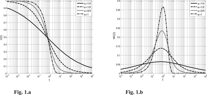
Figure 1. (a) Plots of r(t) with α = 1/4, 1/2, 3/4, 1. (b) Plots of tK(t) withα = 1/4, 1/2, 3/4, 1.
Download figure:
Standard image High-resolution imageBy changing the variable in equation (1), carrying out the integration by part, and substituting equation (2) into equation (1); equation (1) can be recast as follows
where ![${\mathbf{S}}^{\left(\mathrm{e}\right)}\left[\mathbf{C}(t)\right]$](https://content.cld.iop.org/journals/0965-0393/30/3/035003/revision2/msmsac3dd1ieqn23.gif) is the immediate contribution (elastic behavior) as it supports the contribution of the deformation at actual time, and
is the immediate contribution (elastic behavior) as it supports the contribution of the deformation at actual time, and  is the viscous stress.
We note that the integral terms depend on the past history of the material, and the viscous stress is expressed as the sum of three components. The first integral of equation (3) represents a coupling between hyperelasticity (the material nonlinearity) and relaxation. Thereby, in a relaxation test, when time is tending towards 'infinity', the stress response at the equilibrium state is ![${\mathbf{S}}^{\left(\mathrm{e}\right)}\left[\mathbf{C}(t)\right]$](https://content.cld.iop.org/journals/0965-0393/30/3/035003/revision2/msmsac3dd1ieqn25.gif) . As a consequence, this stress is meaningful for the long term highlighting the equilibrium stress. The second integral of equation (3) arises from the so-called fading memory; it represents the instantaneous elasticity at zero-time. We recall that the principle of fading memory was introduced by Coleman and Noll [66] in the sense that the current or recent configurations have a much greater influence on the present state of stress than configurations that existed in the distant past. Valanis [67] showed that fading memory is a consequence of the positive rate of irreversible entropy production. Haupt and Lion [48] proved that the relaxation function of the Mittag–Leffler is consistent with fading memory concept in agreement with the theory of Truesdell and Noll [68]. Moreover, the exponential function for the relaxation is compatible with the principle of thermodynamics.
. As a consequence, this stress is meaningful for the long term highlighting the equilibrium stress. The second integral of equation (3) arises from the so-called fading memory; it represents the instantaneous elasticity at zero-time. We recall that the principle of fading memory was introduced by Coleman and Noll [66] in the sense that the current or recent configurations have a much greater influence on the present state of stress than configurations that existed in the distant past. Valanis [67] showed that fading memory is a consequence of the positive rate of irreversible entropy production. Haupt and Lion [48] proved that the relaxation function of the Mittag–Leffler is consistent with fading memory concept in agreement with the theory of Truesdell and Noll [68]. Moreover, the exponential function for the relaxation is compatible with the principle of thermodynamics.
In order to describe the frequency dependence properties of rubber-like materials, the evolution of material microstructure can be incorporated using the concept of intrinsic time, so-called, z(t) which is driven by the deformation history but not by temperature. Indeed, for thermo-rheological simple materials, the physical meaning of shift time arises from the TTS (time-temperature superposition) principle. The latter states that the effects of time and temperature on the mechanical properties of a viscoelastic material are equivalent [69]. Notice that McGuirt and Lianis [70] generalized the concept of thermo-rheological simple materials to finite deformations in the framework of the theory of thermodynamics of materials with memory.
As a result, we replace the physical time variables, t and s by the variables z and x, [31, 71, 72], and equation (3) becomes
where  .
.
The intrinsic time variable z(t) depends on the structural variable, so-called q(t) as follows

where b ⩾ 0 is a material parameter.
The variable q(t) is a phenomenological measure in the current state of the material's microstructure, which is determined by the evolution equation [31]

with the initial condition q(0) = 0 and  .
.
According to Lion [73], the parameter ς > 0 is a relaxation time that describes the dynamic behavior of the material's microstructure, and the constant τ = 1 s is introduced for dimensional reasons.
The evolution law given by equation (5) is assumed to be linear function of a structural variable q(t). A more general differential equation was used in [51, 56] governing the intrinsic time

where k = 1, ...‥, M.
The solving of equation (7) could require long computation times [56]. Also, it is difficult to provide physical mechanisms justifying a relatively large number of model parameters.
3. Linearization of the model
Let us linearize the constitutive equation in the neighborhood of a static pre-deformation. Following Lion and Kardelky [31], the deformation gradient can be decomposed into a time-independent and a time-dependent part (see figure 2):

where F0 and f(t) are respectively the static part and the dynamic part of the deformation gradient; F0 = const, f(t) = I + h(t) and the magnitude of the incremental displacement gradient h is assumed to be sufficiently small, so  .
.
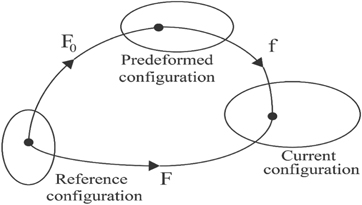
Figure 2. Different configurations.
Download figure:
Standard image High-resolution imageWe note R the difference between a second order tensor Y and his linearization form, we have  for δ → 0 and we write
  , where
  is the Landau symbol [31].
Based on these assumptions, the linearization of all kinematical tensors reads as


where  ,
,
 ,
,
 and
and  is the incremental strain tensor.
The linearization version of the evolution equation (6) is given by

The elastic potential of Mooney–Rivlin is considered in the constitutive model of equation (1), so

where  is the shear modulus at infinitesimal deformations and 0 < χ ⩽ 1 is a dimensionless constant; if χ = 1 then the neo-Hookean model is recovered.
The Cauchy stress tensor can be inferred from equation (4) as follows

where


The second term i.e.
σ
(1)(t) of the constitutive equation embedded both the transient and steady-state responses; the long-term viscous stress (the term for fading memory), i.e.
σ
(2)(t) depends on the strain rate of the superposed state and the overall effect of the past history of the material, whereas r(t) is actually a relaxation function, which could be related to the rearrangement of polymer chains. Indeed, the transient network theory of Tanaka and Edwards [74] states that polymeric chains are divided into permanent networks and transient ones, the latter being rearranged upon deformation. Therefore, the number of chains (active) that contribute to the polymeric network has evolved with time. Accordingly, the viscoelastic response is related to the rearrangement of polymer chains, that is, detachment of active chains or attachment of dangling chains to temporary junctions. Noting that the stress relaxation time is longer compared to the time it takes for the internal microstructure to rearrange. The stress
σ
(3)(t) shows a coupling between the integral term and the material nonlinearity arising from the Mooney Rivlin model  . This stress could be related to the free-fluctuating of the deformed network due to the applied pre-strain. Recalling that the elastic and relaxation responses of a deformed rubber are a priori physically distinct, the former being caused by a change in the equilibrium configuration free energy of the rubber network and the latter being associated with the kinetics of network chain configuration rearrangements.
For sufficiently large times (in stationary state), practically t tends to infinity, so that and equation (18) becomes
The linearization of the first invariant scalar of the tensor C is as follows

Using these approximations and omitting the higher-order terms in the displacement gradient, we may obtain the linearized version of the constitutive equation with respect to the intrinsic time as follows
We observe that the 'equilibrium' stress  is a sum of the static equilibrium stress, i.e.
  that depends only on the pre-deformation, i.e. F0
and of the incremental part of the equilibrium stress, i.e.
that depends only on the pre-deformation, i.e. F0
and of the incremental part of the equilibrium stress, i.e.  , which represents the coupling effects of the basic state and superposed state at the instant t. Pointing out that
  and
and  have been highlighted based on another theory [51]. The stress arising from the first integral depends on the past history of the material, the strain rate, and the strain-energy density. The second integral term depends on the strain rate and the past history of the material as in linear viscoelasticity.
4. Computation of the dynamic complex moduli
Let us consider the simple tension test defined by the deformation gradient

where λ(t) is the stretch ratio.
The deformation gradient F0 of the static pre-deformation and the incremental deformation gradient f(t) are respectively given by

and

then

and

The linearization of  , which leads to the following set of equations


Under simple tension (or compression), the Cauchy stress tensor is given by

We obtain by substituting the equations (26), (27) and (29)–(31) into equation (22):
By eliminating the Lagrange multiplier, i.e. p, we may obtain the Cauchy stress
We will consider the first Piola–Kirchhoff tensor acting on the statically pre-deformed configuration as follows

In the case of simple tension, we have

So
Let us evaluate equation (37) for stationary sinusoidal excitations in the form

where ω is the angular frequency and Δɛ the strain magnitude  .
.
Inserting equation (30) into equation (16), we obtain the one dimensional formulation of the evolution equation

According to Lion and Kardelky [31], the solution of equation (39) is

Inserting equation (40) into equation (5), and after integration, we obtain the intrinsic time variable

Noticing that z(t) is a linear function of time and dynamic amplitude, but nonlinearly depends on the frequency.
Let us develop equation (37) by substituting equation (41) into the Green function  as follows

where τ0 = τR/a.
As a result, we obtain
After calculations, we get
Equation (44) can be written as follows

The first term of equation (45) represents the static stress due to the static pre-deformation λ0, whereas the second term is the dynamic response depending on λ0, ω and Δɛ. So, the storage and loss moduli are given by
and
where

Consequently, both the storage and the loss moduli depend on the magnitude of pre-strain in the case of Mooney–Rivlin model.
For the neo-Hookean model, i.e. c01 = 0, we get
and

For this case, the loss modulus, i.e. E'' does not depend on the static pre-deformation, i.e. λ0. We recall that the complex moduli in [31] arise from solving a fractional differential equation (with respect to the time variable) governing the overstress, which requires many computations. However, the proposed description was proved to be more flexible because it necessitates fewer computations and the Lion and Kardelky model [31] could be recovered.
Following Nashif et al [37], we may introduce the loss factor of the material, i.e. as follows

We may observe that, if λ0 → 1, we then get

The real and imaginary parts of the harmonic complex Young's modulus E* can be inferred from equations (46) and (47) by setting λ0 = 1. As a result, the strain-dependence of harmonic moduli that arises from this approach could be compared, for instance, with moduli in [26]; however, it does not the scope of this paper.
Let us consider the loss factor that is given by
where


and Ωn = ωτR/a.
Figure 3 shows the plots of the loss factor without the Payne effect, i.e. a = 1 and Ωn = ωτR = Ω in the framework of tension and compression mode loadings. In tensile mode, the predictions seem to be qualitatively consistent with the results of [37]. The loss factor decreases with increasing the amplitude of pre-deformation. It can be seen that the plots representing the loss factor are shifted by increasing the pre-strain; to our knowledge, this result was not highlighted in the literature. In compression, the loss factor decreases significantly due to stiffening of the material; the material seems to be stiffening more in compression. Besides, we will consider the influence of the Payne effect a ≠ 1 on the loss factor in the next section.
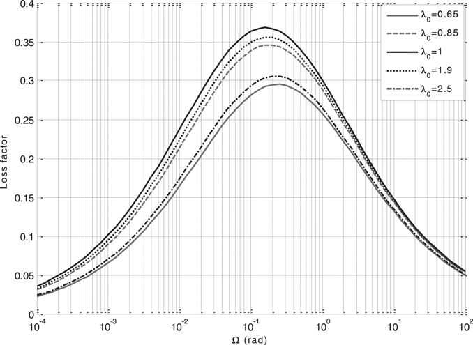
Figure 3. Variation of the loss factor with adimensional frequency Ω and pre-deformation λ0
 .
.
Download figure:
Standard image High-resolution image5. Parameter identification and verification of the model
To check the proposed model's capability of simulating the Payne effect, experimental data of Lion and Kardelky [31] and of Peng et al [36] have been used. Lion and Kardelky [31] have performed their experimental tests on CBR, the testing temperature was about 283 K and the pre-strain was ɛ0 = −0.1. The magnitude of harmonic excitation of small magnitude varied between 0.1% and 5%, and the frequency between 10 Hz and 60 Hz. Peng et al [36] used a dynamic mechanical analyzer to measure the complex Young's modulus of chloroprene rubber (CR). The specimens were pre-stretched sinusoidally with an amplitude λ0 = 1.05 at various frequencies (1–30 Hz), the dynamic amplitude ranges from 0.1% to 3%, and the temperature is 296 K.
The linearization of the model is based on the assumption that the magnitude of the incremental displacement gradient h is small in comparison to 1, i.e. δ ≪ 1.
The maximum value of the norm of h(t) is given by

The maximum value of the magnitude of harmonic excitation is Δɛ = 0.05 and we have ![$\mathrm{sin}\left(\omega t\right)\in \left[-1,\enspace 1\right]$](https://content.cld.iop.org/journals/0965-0393/30/3/035003/revision2/msmsac3dd1ieqn49.gif) , then
, then ![$\delta =\mathrm{max}\left({\left[{\left({\varepsilon }_{L}(t)\right)}^{2}+2{\left(\frac{1}{\sqrt{1+{\varepsilon }_{L}(t)}}-1\right)}^{2}\right]}^{1/2}\right)\approx 0.0621$](https://content.cld.iop.org/journals/0965-0393/30/3/035003/revision2/msmsac3dd1ieqn50.gif) . which can be neglected in comparison to 1
. which can be neglected in comparison to 1
In these tests, the equilibrium state is assumed to be reached after a sufficiently long time (when the Mullins effect is removed), and before applying dynamic small vibrations on the specimen. We first observe that the material constants c10 and c01 may, in principle, be determined from simple tension tests or/and equi-biaxial tension tests under the quasi-static conditions [75, 76]. These constants should be valid to characterize the multi-axial mechanical behavior in the steady-state. Thus, it is difficult to determine the material constants c10 and c01 from experimental data of the simple tension tests, which are performed in the pre-deformed configuration. It should be pointed out that both equilibrium and instantaneous responses are elastic and are linked to the viscosity domain. As a result, the present identification would induce imprecision on the values of these material parameters. Notice that an agreement with the uni-axial test data does not guarantee that the proposed model will correctly predict actual material behavior for multi-axial stress fields. For this reason, a biaxial test needs to be performed in order to obtain experimental data, which could be used to validate the model predictions. In fact, for incompressible materials, the biaxial test is the most general since any triaxial stress state may be reduced to a biaxial one (without changing the state of deformation) by the superposition of an appropriate hydrostatic pressure [77]. Besides, the relaxation function r(t) does not depend on the pre-stretch, i.e. λ0. However, for filled rubbers, experiments show that the relaxation depends on the static deformation [78]. Thereby, a correction factor was introduced in order to account for the non-separability of time and deformation in the relaxation function [34].
The material parameters were estimated by using the standard minimization technique. To this end, one needs to define the objective function  as the quadratic squared sum of the residuals, i.e. the difference between the experimental moduli data and the corresponding theoretical values:
where M and M' are the numbers of data points,  the unknown parameters set, and
  and
and  are the theoretical moduli and computed according to equations (46) and (47). The weighted factors w1 and w2 are introduced in order to properly scale the residuals terms, i.e.
  and
and  . When the two residual terms have different orders of magnitude, the values of weight factors should not be equal. It can be seen that the magnitude of the dissipation modulus is approximate to 1/3 for [31] and to 1/4 for [36] of that of the storage modulus. So, the weighting factors are chosen as w1 = 1, w2 = 3 and w1 = 1, w2 = 4, respectively. The minimization problem consists of

With  the solution space,
  and
and  are the lower and upper bounds, respectively. The physical values of each material parameter were estimated to define the bounds of the vector
  .
.
Noting that global optimization or gradient-based local optimization methods are often used to calibrate the hyperelastic model constants [79, 80]. Apart from gradient-based methods, other gradient-free schemes are applied, for example, neural networks [81] or with a direct search method [82]. To obtain the model parameters of equation (54), we use a nonlinear least-square method (NLS), which requires an initial guess for the solution. We follow the gradient-based local optimization method, the objective function  is minimized using the Lsqcurvefit implemented in the Optimization Toolbox of Matlab, and it is called the function fmincon and Lsqcurvefit. For instance, the combination of the Lsqcurvefit function and the trust-region-reflective method was used in the framework of visco-hyperelasticity [60] to obtain an optimal model parameter set corresponding to a global optimum. Accordingly, we have used a multi-start approach to running the optimization function with varying initial guesses. To this end, each parameter of the model should be bounded based on physical arguments, so that

The constants of hyperelastic models must be determined carefully to obtain stable constitutive equations for all deformation states, and so to avoid numerical instabilities. Reasonable restrictions on material parameters based on physical arguments seem to be an unsolved question. Several inequalities such as the Backer–Ericksen inequalities, Coleman–Noll inequalities, strong ellipticity, polyconvexity, etc, have been proposed in the literature. The reader may refer to a recent paper for details [83]. Practically, we can assume that the model constants must meet the Drucker-stability criterion, i.e. the fourth-order elasticity tensor must be positive definite. Consequently, the choice for stable Mooney Rivlin model constants would be choosing them to be positive-valued [84]. Recently, Upadhyay et al [83] have proved that this choice is consistent based on the so-called T–C inequality. As a result, in equation (17), the Mooney Rivlin's constants are positive-valued. Moreover, for soft materials, the shear modulus is of the order of a few MPa, so that, we may assume that its upper value is 10 MPa, therefore;  . Note that the material parameters μ0 and χ must be determined from the data of both simple tension and equi-biaxial tension (or compression test).
The fractional derivatives theory imposes the values of the real number  and we have
  [63]. We note that the relaxation behavior of filled rubbers is characterized by a very rapid decrease of the stress at the beginning of a hold time, followed by an extremely slow decay during several hours [71]. So, the values of the relaxation time, i.e. τR are assumed to be in the range of 10−3 s to 60 s. Moreover, the values of the material parameter b must be delimited; Lion and Kardelky [31] have estimated b of the order of 5 × 10⁴. We choose the upper bound for the parameter b equal to 109 which can be considered a very great value (see appendix
The 'best' solution  is that corresponding to the globally minimum. Practically, the number of 3000 iterations has been performed, and it was assumed as a criterion of the convergence to quasi-unique and 'stable' model parameters.
The quality of the solution is validated by computing the root-mean-square (RMS) as follows

The RMS gives indications on how the model reproduces the experimental data. However, we cannot say anything about the quality of the parameters found [85]. Notice that the previous boundings exclude a priori to find numerical values without physical meanings of the model parameters.
Both the RMS corresponding to the storage and dissipation moduli were computed for each frequency. It is worth noting that, the experimental data used in this study are available in the literature. The determined values of material parameters are listed in tables 1 and 2, whereas the fitting results are shown in figures 4(a)–7(a). Figures 4(b)–7(b) show the relative error versus strain amplitude for different values of frequency. The storage and loss moduli give qualitatively good results concerning the shape of the two curves versus the strain magnitude and the frequency. These figures show that the storage modulus i.e.  decreases monotonously with strain, i.e. Δε, while the loss modulus, i.e.
  displays a non-monotonic variation. Hence, they reflect the influence of the Payne effect. For the results of Kardelky and Lion, the worst fit for the loss modulus was achieved for low magnitudes of the dynamic strain Δɛ ⩽ 0.3% and low frequencies, i.e. 10 Hz–20 Hz, while the RMS for the storage modulus does not exceed 12%. For the results of Peng et al, the error is less than 20%. These high percentages of error arise from the linearity of the differential equation governing the intrinsic time variable.
Table 1. Identified material parameters: experimental data of Lion and Kardelky (2004).
| Parameter | μ0 (MPa) | χ | ξ | α | β | τR (s) | b |
|---|---|---|---|---|---|---|---|
| Value | 1.956 | 0.707 | 0.179 | 0.451 | 0.249 | 59.997 | 3542 485.04 |
Table 2. Identified material parameters: experimental data of Peng et al (2020).
| Parameter | μ0 (MPa) | χ | ξ | α | β | τR (s) | b |
|---|---|---|---|---|---|---|---|
| Value | 1.897 | 0.603 | 0.188 | 0.349 | 0.424 | 0.0036 | 236.22 |
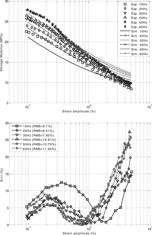
Figure 4. (a) Storage modulus versus dynamic strain: comparison among different frequencies with experimental data of Lion and Kardelky (2004). (b) Relative error of storage modulus versus dynamic strain for different values of frequency: experimental data of Lion and Kardelky (2004).
Download figure:
Standard image High-resolution image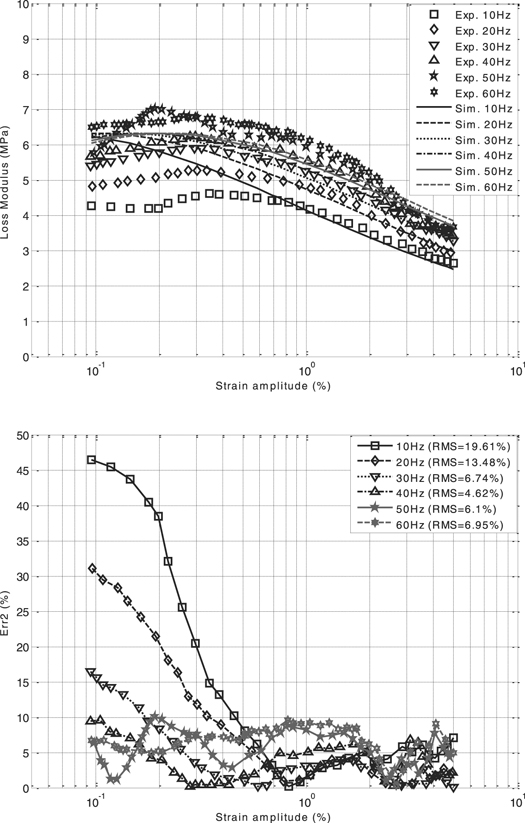
Figure 5. (a) Loss modulus versus dynamic strain: comparison among different frequencies with experimental data of Lion and Kardelky (2004). (b) Relative error of loss modulus versus dynamic strain for different values of frequency: experimental data of Lion and Kardelky (2004).
Download figure:
Standard image High-resolution image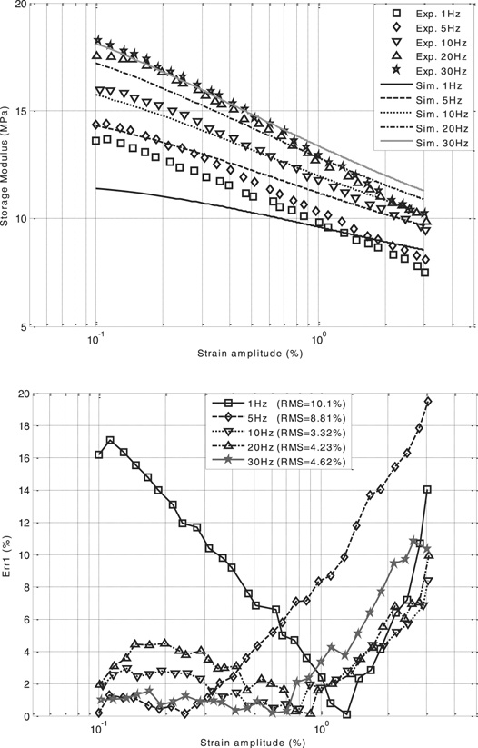
Figure 6. (a) Storage modulus versus dynamic strain: comparison among different frequencies with experimental data of Peng et al (2020). (b) Relative error of storage modulus versus dynamic strain for different values of frequency: experimental data of Peng et al (2020).
Download figure:
Standard image High-resolution image
Figure 7. (a) Loss modulus versus dynamic strain: comparison among different frequencies with experimental data of Peng et al (2020). (b) Relative error of loss modulus versus dynamic strain for different values of frequency: experimental data of Peng et al (2020).
Download figure:
Standard image High-resolution imageTo improve the predictions of the storage and loss moduli, a nonlinear differential equation can be used for the intrinsic time. Therefore, the number of the model parameters must increase, and the computation of the moduli becomes very complicated (see appendix
For the data of Lion and Kardelky (2004), the investigated storage and loss moduli show that the RMS is found between (7.92%–11.55%) and (4.62%–19.61%) respectively. For the data of Peng et al (2020), the RMS of storage and loss moduli are varied respectively between (3.32%–10.1%) and (3.92%–10.74%). It can be seen that a relatively good agreement was obtained between theory and experiment.
Let us consider the influence of the Payne effect a ≠ 1 on the loss factor.
We have Ωn
= ωτR/a where  and ω = 2πf is the radial frequency.
The plots of η versus log Ωn are displayed in figures 8(a) and (b) for the two extreme values of the frequencies used in their experiments, i.e. 10 Hz and 60 Hz for the results of Lion and Kardelky (2004) and 1 Hz and 30 Hz for the results of Peng et al (2000). The curves seem to reproduce the master curve that can be compared to that from arising by varyingtemperatures.
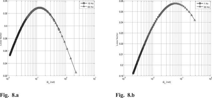
Figure 8. (a) Variation of the loss factor with adimensional frequency Ωn : the material parameters of CBR (Lion and Kardelky (2004)). (b) Variation of the loss factor with adimensional frequency Ωn : the material parameter of CR (Peng et al (2020)).
Download figure:
Standard image High-resolution imageWe recall that the data of uni-axial tensile alone are used for the calibration of the model parameters. As a result, these parameters should not ensure to predict the multi-axial stress state. Hereafter, the same set of model parameters was used to predict the first Piola–Kirchhoff stress in the pre-deformed configuration, i.e. equation (44). The plots are shown in figures 9 and 10 for the compression loading and in figures 11 and 12 for the tensile loading, the trends of the results reproduce the experimental data and seem to be qualitatively satisfactory and conforming with the results of the literature [56].
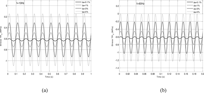
Figure 9. Stress-time curves with different dynamic strain amplitudes at 10 Hz (a) and 60 Hz (b).
Download figure:
Standard image High-resolution image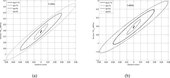
Figure 10. Stress–strain curves with different dynamic strain amplitudes at 10 Hz (a) and 60 Hz (b).
Download figure:
Standard image High-resolution image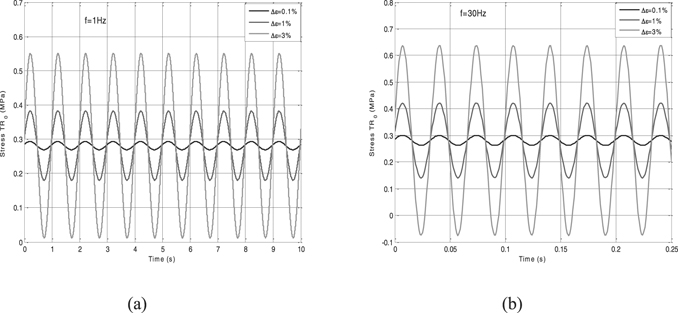
Figure 11. Stress-time curves with different dynamic strain amplitudes at 1 Hz (a) and 30 Hz (b).
Download figure:
Standard image High-resolution image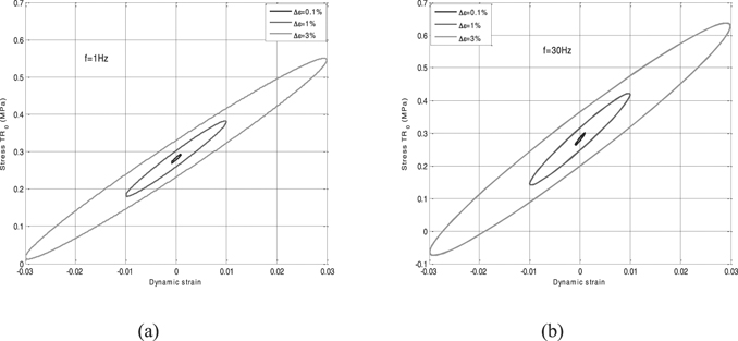
Figure 12. Stress–strain curves with different dynamic strain amplitudes at 1 Hz (a) and 30 Hz (b).
Download figure:
Standard image High-resolution image6. Conclusion
In this work, the Payne effect has been modeled based on the visco-hyperelastic model presented and analyzed in previous work. The proposed model was formulated on the grounds of the concept of dual variables in the framework of extension of the fractional constitutive equation of the SLS to finite strains. So, the proposed constitutive equation seems to include the Lion and Kardelky model as a special case. The present model was used to evaluate the harmonic complex Young's modulus with regards to the Payne effect. To this end, experimental data of literature were employed to check the model's capability. Indeed, the model was calibrated from experimental data of compression and tensile loading tests, which were performed for a pre-deformation, a wide range of frequencies, and small harmonic strains that were superimposed on a steady state. We have shown that the proposed description is more flexible, given that the computation is easier. Thereafter, the same set of parameters identified from the storage and loss moduli was used to predict the stress in the pre-deformed configuration. The present modeling has certain accuracy in predicting the Payne effect. Hence, the proposed constitutive equation could be suitable for modeling the mechanical behavior of unfilled rubbers. To improve the predictions of the storage and loss moduli, a nonlinear differential equation can be used for the intrinsic time. Therefore, the number of the model parameters must increase, and the computation of the moduli becomes very complicated. So, a balance should be found between the flexibility of the calculation of moduli and the type of differential equation. Besides, the predictions of the present model can be improved by considering the effect of pre-stretch on the relaxation function. The present model can also be implemented in FE codes in order to simulate the response of materials and structures.
Acknowledgments
We would like to thank the anonymous Reviewers for their detailed comments, which have significantly improved the content of this paper.
Data availability statement
All data that support the findings of this study are included within the article (and any supplementary files).
Appendix A
The procedure of calibration of optimal model parameters is based on the gradient-based local optimization method. Therefore, the objective function is minimized by using the Levenberg–Marquardt algorithm implemented in the Optimization Toolbox of Matlab, and it is called the function fmincom and lsqcurvefit. Then, multi-start approaches, i.e. different initial guesses were used to obtain the global optimal parameter set.
We have chosen the Latin hypercube sampling procedure to generate N starting guesses. To do this, each parameter of the model should be bounded based on physical arguments. The values of the positive material parameter b must be delimited, so we write

In order to find a global solution, we have used the lsqcurvefit function of Matlab together with MultiStart by varying initial guesses. The lhsdesign (N, 7) is used to generate a Latin hypercube sampling that contains N values of each of the seven (7) parameters. The N values of each colon of the matrix T are randomly distributed with one from each interval (0, 1/N), (1/N, 2/N), .........((N − 1)/N, 1). We create a matrix A that contains N initial guesses as follows

where lbij and ubij represent respectively the lower and upper bound for a parameter κj .
We execute multiStart using the lsqcurvefit function as the local solver with N initial guesses given by the matrix A. The iterations of the NLS algorithm can stop when the number of iteration surpasses 3000.
The tables A.1 and A.2 give, respectively, the identified parameters of the experimental data of Lion and Kardelky (2004) and of Peng et al (2020) for N = 10, N = 100, N = 1000,N = 3000.
Table A.1. Identified material parameters for experimental data of Lion and Kardelky (2004).
| N | ||||
|---|---|---|---|---|
| Parameter | 10 | 100 | 1000 | 3000 |
| μ0 (MPa) | 2.029 | 2.073 | 2.055 | 1.956 |
| χ | 0.871 | 0.970 | 0.931 | 0.707 |
| ξ | 0.181 | 0.183 | 0.182 | 0.179 |
| α | 0.451 | 0.451 | 0.451 | 0.451 |
| β | 0.249 | 0.249 | 0.2495 | 0.249 |
| τR (s) | 59.973 | 59.994 | 59.999 | 59.997 |
| b | 3540 105.40 | 3542 360.71 | 3542 633.25 | 3542 485.04 |
Table A.2. Identified material parameters for experimental data of Peng et al (2020).
| N | ||||
|---|---|---|---|---|
| Parameter | 10 | 100 | 1000 | 3000 |
| μ0 (MPa) | 1.904 | 1.937 | 1.919 | 1.897 |
| χ | 0.567 | 0.392 | 0.486 | 0.603 |
| ξ | 0.190 | 0.201 | 0.195 | 0.188 |
| α | 0.349 | 0.349 | 0.349 | 0.349 |
| β | 0.424 | 0.424 | 0.424 | 0.424 |
| τR (s) | 0.0036 | 0.0036 | 0.0036 | 0.0036 |
| b | 236.23 | 236.21 | 236.23 | 236.22 |
We can see that we find a similar value of these parameters  for different values of iterations but different values for
  , this latter may be determined under the quasi-static conditions.
We have identified the model parameters by considering other values for the upper bound of the parameter τR and the number of iterations is taken as N = 3000.
Let us consider the error R0 that is defined by
where m represents the number of frequencies used in the test.
The plots of the error R0 are shown in figure A.1 versus the value of the upper bound of the relaxation time, i.e.  , in the framework of both the Kardelky and Lion and of Peng et alresults.

Figure A.1. Plots of R0 versus  : the results of Kardelky and Lion (a) and the results of Peng et al (b).
Download figure:
Standard image High-resolution image
The graph of figure A.1(a) shows that the function R0 decreases for the low values of  and it remains quasi-constant for
  . In figure A.1(b), the variation of values of
  do not affect the error R0.
In tables A.3 and A.4, we present a comparison between the numerical values of material parameters that arise from identification and of the values of RMS in the context of choosing two upper bounds for the relaxation time,  and
and  .
.
Table A.3. Comparison of the consistency of computed numerical values of material parameters depending on the value of  .
.
| Kardelky and Lion results | Peng et al results | ||||
|---|---|---|---|---|---|
| Parameters |

|

| Parameters |

|

|
| μ0 (MPa) | 1.956 | 2.042 | μ0 (MPa) | 1.897 | 1.941 |
| χ | 0.707 | 0.903 | χ | 0.603 | 0.375 |
| ξ | 0.179 | 0.182 | ξ | 0.188 | 0.202 |
| α | 0.451 | 0.451 | α | 0.349 | 0.349 |
| β | 0.249 | 0.249 | β | 0.424 | 0.424 |
| τR (s) | 59.997 | 399.994 | τR (s) | 0.0036 | 0.0036 |
| b | 3542 485.04 | 23 619 428.21 | b | 236.22 | 236.23 |
Table A.4. Comparison of the consistency of computed numerical values of RMS depending on the value of  .
.
| RMS (E', E'') % Kardelky and Lion results | RMS (E', E'') % Peng et al results | ||||
|---|---|---|---|---|---|
| Frequency (Hz) |

|

| Frequency (Hz) |

|

|
| 10 | (9.10, 19.61) | (9.10, 19.61) | 1 | (10.10, 3.92) | (10.10, 3.92) |
| 20 | (8.41, 13.48) | (8.41, 13.48) | 5 | (8.81, 10.74) | (8.81, 10.74) |
| 30 | (7.92, 6.74) | (7.92, 6.74) | 10 | (3.32, 7.47) | (3.32, 7.47) |
| 40 | (10.91, 4.62) | (10.91, 4.62) | 20 | (4.23, 9.59) | (4.23, 9.59) |
| 50 | (10.75, 6.1) | (10.75, 6.1) | 30 | (4.62, 10.63) | (4.62, 10.63) |
| 60 | (11.55, 6.95) | (11.55, 6.95) | |||
One can see that the values of the parameters b and τR are sensitive on choosing the value of  in the framework of Kardelky and Lion results, but their ratio, i.e. b/τR ≈ 5.90 × 10⁴ s−1 is quasi-constant. Noting that the RMS values of both the storage and loss moduli do not depend on the value of
  . However, no difference was highlighted in analyzing the Peng et alresults.
Let us consider the expressions of the storage and loss moduli equations (46) and (47) in order to explain in depth the difference arising from Kardelky and Lion results and Peng et alresults.
We recall that the storage and loss moduli are functions of the variable ωτ0 that is defined by  .
.
If  then we obtain
  .
.
As a result, the variable ωτ0 depends on the ratio  .
.
For the ratio corresponding to the Kardelky and Lion results, the values of parameters b and τR cannot be unique.
Otherwise, if  is not negligible compared to
 , the values of the parameters b and τR seem to be stable, that is the case of the results of Peng et al for which the results do not depend on the value of
  .
.
: Appendix B
In experimental testing, the material behavior of filler-reinforced rubber under dynamic deformation shows a weakly dependence on the frequency of deformation but a pronounced dependence on the dynamic strain amplitude. This well known Payne effect can be described as follows
- Increasing frequency f leads to an increase in the storage and loss moduli,
- The storage modulus decreases with increasing dynamic strain amplitude while the loss modulus runs through a distinct maximum.
Mathematically, we can write

and
where Δɛ0,f represents the value of strain amplitude in which the loss modulus is maximum.
The storage and loss moduli given by equations (46) and (47) depend on seven parameters and we have

and

where

and
For any value of parameters  , we have

For the loss modulus, we have
and

where

It can be seen that if  , i.e.
 ![$\left[1-{\left(\omega {\tau }_{0}\right)}^{2\alpha }\right] > 0$](https://content.cld.iop.org/journals/0965-0393/30/3/035003/revision2/msmsac3dd1ieqn99.gif) , implies that
, implies that .
.
Then, if we impose the constraint of monotonicity of loss modulus versus frequency, the loss modulus decreases with dynamic strain amplitude which disagrees with the experiment. It can be concluded that for the present model, the two conditions cannot be verified simultaneously for low dynamic strains.
If we consider another type of evolution equation to represent the process dependence of the Payne effect, for example, the evolution equation for the rate of the intrinsic time given in [51] or in [56]:


where 0 ⩽ δ ⩽ 1, and 0 < γ ⩽ 1.
The computation of the storage and loss moduli becomes very complicated and the number of material parameters increases.
In order to illustrate the effect of incorporation of the first term of equation (B.10) in the evolution equation for the rate of the intrinsic time, we consider a special choice given by equation (B.10a).
In the expression of the stress TR0 (equation (37)), we can replace the integral term

by the differential equation

where

We note that the equation (B.11) is the solution for the fractional differential equation (B.12) in the stationary state.
This differential equation is formulated with reference to a new time scale z, which can either evolve faster or slower than the real time t, this formulation is also equivalent to a varying relaxation time in equation (B.12) [51].
We assume that
and the differential equation (B.12) becomes

To calculate the dynamic moduli of the proposed model with the hypothesis of the effective relaxation time equation (B.14), we assume the stationary sinusoidal deformation

We have

and

We use the method of Galerkin to calculate the functions A and B

For  and
and  , we obtain a system of linear equations for the functions A and B
After calculations, we obtain
where

Solving these equations, we obtain
As a result, the dynamic moduli are given by
If δ = 0 and l = 1 then, we obtain c = bq + 1 = a and 
In this case, the dynamic moduli reduce to the equations (46) and (47)
An equilibrium between the flexibility of the moduli's computations and the differential equation of the evolution law should, therefore, be found.