

Abstract
Unsteady inlet flow distortion can influence the stability and performance of any propulsion system, in particular for more novel, short and slim intakes of future aero-engine configurations. As such, the requirement for measurement methods able to provide high spatial resolution data is important to aid the understanding of these flow fields. This work presents flow field characterisations at a crossflow plane within a short aeroengine intake using stereoscopic particle image velocimetry (SPIV). A series of tests were conducted across a range of crosswind and high angle of attack conditions for a representative short and slim aspirated intake configuration at two operating points in terms of mass flow rate. The velocity maps were measured at a crossflow plane within the intake at an axial position L/D = 0.058 from where a fan is expected to be installed. The diameter of the measurement plane was 250 mm, and the final spatial resolution of the velocity fields had a vector pitch of 1.5 mm which is at least two orders of magnitude richer than conventional pressure-based distortion measurements. The work demonstrates the ability to perform robust non-intrusive flow measurements within modern intake systems in an industrial wind tunnel environment across a wide range of operating conditions; hence, it is suggested that SPIV can potentially become part of standard industrial testing. The results provide rich datasets that can notably improve our understanding of unsteady distortions and influence the design of novel, closely coupled engine-intake systems.
Export citation and abstract BibTeX RIS

Original content from this work may be used under the terms of the Creative Commons Attribution 4.0 license. Any further distribution of this work must maintain attribution to the author(s) and the title of the work, journal citation and DOI.
Nomenclature(s)
List of symbol
| α | Incidence angle |
| D/R | Diameter/Radius of inlet |
| Dspinner/Rspinner | Diameter/Radius of spinner |
| Dhi | Diameter of intake highlight plane |
| δ | droop angle |
| f | Focal length of lens |
| f# | F-stop of the lens |
| h | Vertical distance between ground board and lower-lip highlight |
| s | Curvilinear coordinate |

| Model exit mass flow rate |

| Maximum corrected mass flow |
| M∞ | Freestream Mach number |
| V∞ | Crosswind velocity |
| L | Inlet length |
| Wmax | Maximum flowrate |
| dt | Pulse separation time |
| σ | scarf angle |
Abbreviations
| AIP | Aerodynamic Interface Plane |
| DSR | Dynamic Spatial Range |
| DVR | Dynamic Velocity Range |
| DNW | German-Dutch Wind Tunnels |
| PIV | Particle Image Velocimetry |
| SAE | Society of Automotive Engineers |
| SPIV | Stereoscopic Particle Image Velocimetry |
| UHBR | Ultra-High Bypass Ratio |
1. Introduction
The performance and environmental targets are driving the design of next-generation aircraft towards closer integration between the propulsion system and the airframe (Cousins 2004). The next generation of architectures will feature aero engines with higher bypass ratios (i.e., larger diameters) to improve propulsive efficiency and reduce specific fuel consumption (Birch 2000). Such engines may feature short and slim intakes to compensate for the additional aerodynamic drag and weight penalties associated with the increased fan diameter. However, such short intakes can potentially cause high levels of unsteady flow distortion, especially under crosswind and incidence operations (Daggett et al 2003), which can have a detrimental effect on the performance and stability of the downstream turbomachinery (Zhang and Vahdati 2019). The presence of inlet flow distortion directly impacts the aerodynamic loading on the fan blades, reducing the stability margin, and can lead to fan stall events (Stenning 1980).
Experiments involving flow field investigations of aero-engine inlets for development, testing and certification activities rely predominantly on intrusive measurement techniques like pressure and temperature rakes (Hodder 1981, Toge and Pradeep 2017). These are mature experimental techniques with well-known limitations, such as intrusiveness and lower spatial resolution. For example, the total pressure is typically measured with 40 pressure probes (Keerthi et al 2017), which cannot perform instantaneous flow measurements and thus infer information on the flow dynamics (Larkin and Schweiger 1992). These measurements cannot capture the complex unsteady flow distortion patterns generated in intake under separated-flow conditions, where high spatial resolution and synchronous instantaneous measurements are highly advantageous (Gil-Prieto et al 2019). This introduces a potential risk that intake/engine incompatibilities go undetected until later stages of the engine development.
Laser-based optical measurement techniques like Particle Image velocimetry (PIV) can overcome these limitations in the current practices for aero-engine inlet distortion characterisation. This technique provides non-intrusive, instantaneous, synchronous measurements across a large flow field area at a much higher spatial resolution than traditional methods. For example, PIV methods have previously been used to provide about 250 times more data points than conventional experimental techniques based on 40 pressure transducers (Zachos et al 2016). Therefore, stereoscopic particle image velocimetry (SPIV) has the potential to identify and enable earlier evaluation of flow phenomena of interest. This has recently received attention for investigating the flow field in aero-engine intakes (Gil-Prieto et al 2019). Murphy and MacManus (2011) applied SPIV to investigate the ground vortex generated in an aero-engine intake model (D = 100 mm) under quiescent, headwind and crosswind conditions. Zachos et al (2016) successfully employed SPIV to measure the unsteady flow distortion generated downstream of small-scale S-shaped diffuser models with an aerodynamic interface plane (AIP) diameter of 150 mm; the measurements were taken through a transparent cylindrical section located downstream of the diffuser model. Nelson et al (2014) applied SPIV in an industrial environment to measure artificially generated swirl distortion upstream of a JT15D-1 turbofan engine. However, the measurements were restricted to 45° sectors due to the limited optical access, preventing the analysis of the instantaneous flow field of the complete domain.
The application of stereoscopic PIV for characterising the intake flow poses several technical challenges. Optical distortion through cylindrical walls is a well-known issue (Van Doorne and Westerweel 2007). Obtaining uniform seeding density in the measurement plane is also challenging in large-scale experiments (Guimaraes et al 2018). Finally, despite some successful applications in an academic, bespoke research laboratory environment (Zachos et al 2016), this technique has yet to be demonstrated in industrial, large-scale environments where aero-engine intakes are typically tested.
The current research demonstrates SPIV a mature measurement technique to perform robust, highly automated measurements in an industrial wind tunnel environment for the characterisation of internal flows, pertinent to state of the art civil aero-engine intakes. The experiments were performed for incidence and crosswind configurations for a representative ultra high bypass ratio (UHBR) aspirated inlet (i.e., without a fan). A multicamera (6 sCMOS) SPIV approach was used to measure unsteady flow distortions at a crossflow plane downstream of the intake across the full annulus. The inlet flow is characterised during incidence to determine the angle of attack at which the flow separates for two different mass flow rates. Under crosswind conditions, both mass flow and velocity sweeps were performed to understand the flow distortion behaviour. The measured three velocity components enable the assessment of the distortion metrics at each SPIV snapshot. The current work demonstrates the ability to perform robust, non-intrusive flow measurements within a UHBR aero-engine intake system in a large scale, industrial wind tunnel environment.
2. Experimental setup and methods
2.1. Wind tunnel and model instrumentation
The experiments were conducted in the low-speed tunnel (LST) of the German-Dutch wind tunnels (DNW). The LST is an atmospheric closed-loop low-turbulence wind tunnel. It features a 9:1 contraction and a rectangular 3 × 2.25 m2 test section where a maximum freestream velocity of 80 m s−1 can be achieved. The intake test model used was representative of a modern UHBR configuration with a fan face hub to tip ratio (Dspinner /D) of 0.3 (see figure 1) achieved by the nose cone that was in place. The intake features droop (δ) and scarf angles (σ). Optical access for the laser sheet was provided through a transparent ring, separated by a slit to allow performing PIV measurements at two cross-flow planes upstream of the notional fan face plane separated by 0.04D (figure 1).

Figure 1. Illustration of the turbofan model indicating key geometrical parameters and PIV plane location upstream of the notional fan face (left). View of the test model looking downstream indicating laser plane configurations and total pressure distortion rake (right). Images not to scale.
Download figure:
Standard image High-resolution imageThe intake model was tailored made to facilitate the SPIV measurements. However, a range of additional, more conventional instrumentation was also included, to complement the SPIV measurements, which are reported below for completeness:
- An 8 × 10 rake configuration (8 rakes with 10 total pressure probes each) was used to measure the fan face, time-averaged total pressure distortion (red dots in figure 1-right). The rakes at 0°, 90°, 180° and 270° were further instrumented with a total temperature probe (thermocouple type). The rakes at 90° and 180° had two additional Kulites for dynamic total pressure measurement at these locations.
- 16 static pressure taps were used on the inner cowling behind the PIV slit to provide the circumferential static pressure distributions in the vicinity of the PIV plane (blue dots in figure 1 right). The ring was upstream of the fan face by 0.008D. Pressure taps were located every 22.5° with an offset of 10° from top dead center (blue dots in figure 1 right). In addition, a circumferential ring of 8 pressure taps was installed along the spinner, 0.008D upstream of the fan face location every 45°, with an offset of 10° (yellow dots in figure 1 right).
- To measure the lip static pressure distributions, 10 streamwise pressure sections were installed at 0°, 45°, 67.5°, 90°, 112.5°, 135°, 157.5°, 180°, 202.5°, 270° (Purple marks in figure 1 left). Each section had between 19 and 24 taps.
Two setups were investigated as part of the experiments at incidence and crosswind. For the incidence configuration, the model was mounted on a turntable (indicated in figure 2(a)) and was rotated about the PIV plane (referred to as α) from 0° to 35° for a set camera position. For the crosswind configuration, a ground board was placed at a representative vertical distance (h) of 0.30D from the lower lip highlight, while the model was rotated to 90° (refer to figure 2(b)). The flow direction is into the plane in figures 2(a) and (b) indicated by blue arrows. The model is rotated along the direction indicated in figure 2(a) (red arrow) for the incidence case.

Figure 2. Test section with the test article in place for incidence (a) and crosswind (b) tests. Note: the model in (a) is looking into the flow, the direction of rotation for angle of attack for incedence is shown in the red arrow, laser head (enclosed in red box) mounted underneath the turntable to enabe alignment of the laser sheet with the model (c).
Download figure:
Standard image High-resolution imageThe required mass flow through the inlet was obtained via a system of blowers corresponding to a remote coupled engine/inlet configuration (Hodder 1981). The mass flow system (root blowers) was checked with a calibrated Bellmouth inlet which operates on the principle of Venturi flow meters (Smith 1985), and the errors in the computed mass flow were calculated to be less than 1% of the maximum designed mass flow rate (Wmax).
2.2. PIV setup and methods
For the PIV measurements, a multicamera optical setup with six LaVision Imager sCMOS cameras (2560 × 2160 pixels, 16 bits, and 6.5 µm pixel size) was used. Pre-tests conducted at the wind tunnel facility of TU Delft were used to de-risk the multicamera stereo-PIV approach. As part of these preliminary tests measurements were carried out employing stereo-PIV, tomographic-PIV and Lagrangian Particle Tracking using Shake-The-Box. Results from these experiments will be reported separately. For the measurements in the LST, a set of Nikon lenses with a focal length of 105 mm were employed. Each camera was fitted with an ISEL™ rotation stage and an automatic Scheimpflug to obtain a uniform focus quality and repeatability as the model configuration varied. This system enabled continuous data acquisition for multiple incidence angles and PIV planes without the requirement of manual adjustments. The cameras were placed outside the wind tunnel in two configurations—one for incidence (figure 3(a)) and crosswind conditions (figure 3(b)). Data for α corresponding to 25° to 35° were acquired in the incidence configuration.
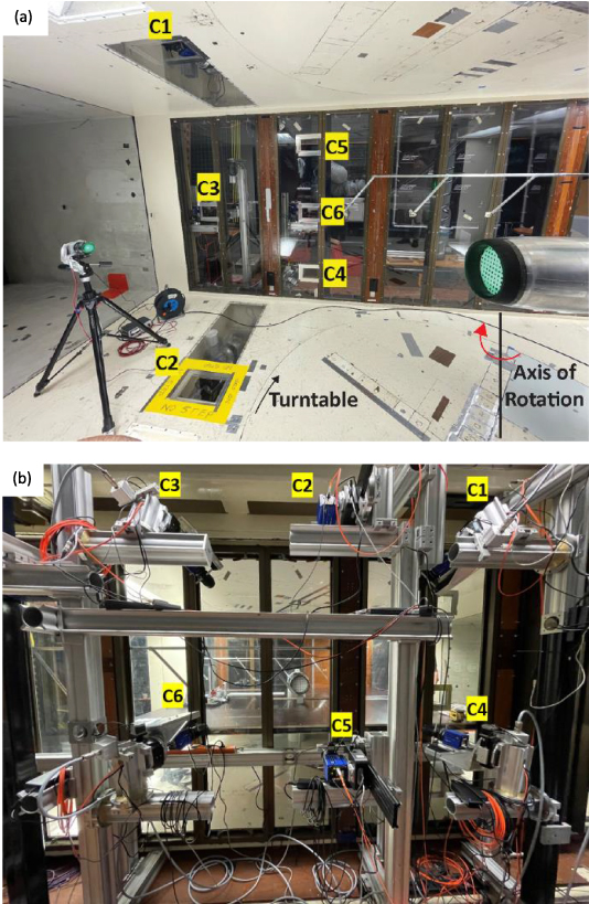
Figure 3. Camera configuration of the 6-camera stereo-PIV system for incidence (a) and crosswind (b) measurements in the DNW Low Speed Tunnel.
Download figure:
Standard image High-resolution imageThe required illumination was provided by two Quantel Evergreen Nd:YAG lasers, which were coupled and mounted on a traverse underneath the turntable (refer to figure 2(c)). The two laser beams, placed at 90° to each other (indicated in the illustration in figure 1), were used to minimise the effect of the shadow produced by the spinner. The automated traverse enabled the translation of the laser sheet from Planes 1 and 2 during data acquisition. The flow was seeded with DEHS particles of 1 µm median diameter. The pulse separation time was chosen to achieve an out-of-plane loss-of-correlation factor (Fo) larger than 0.75 (Keane and Adrian 1993). The experimental parameters are provided in table 1.
Table 1. Specifications of the PIV equipment used.
| Instrument | Description | ||
|---|---|---|---|
| Imaging | Cameras | 6 × LaVision sCMOS (2560 × 2160 pixels, pixel pitch of 6.5 µm, 16 bit) | |
| Recording method | Double frame/Single exposure | ||
| Number of cameras | 6 (C1, C2, C3, C4, C5, C6) Figures 3(a) and (b) | ||
| Recording lens and aperture | 6 × Canon f = 105 mm, f# = 2.8 | ||
| Imaging resolution | Incidence | 7.3 pixels mm−1 | |
| Crosswind | 8.1 pixels mm−1 | ||
| Recording frequency | 15 Hz | ||
| Rotation stage | LaVision ISEL stages | ||
| Automatic scheimpflug | LaVision canon USB scheimpflug | ||
| Illumination | Laser 1 | Quantel evergreen Nd:YAG (2 × 200 mJ at 15 Hz) | |
| Laser 2 | Quantel Evergreen HP Nd:YAG (2 × 340 mJ at 15 Hz) | ||
| Seeding | Tracer particles | Di-ethyl-hexyl-sebacat (DEHS) | |
The cameras were calibrated for each measurement configuration (i.e., each α in the incidence case and the two PIV planes). The camera positions were chosen based on the prior experience in the pre-tests at TU Delft and the optimisation of the camera overlaps, which were analysed from CAD views of the test environment. The calibration was performed in three steps. Initially, the Scheimpflug axis was adjusted using the ISEL™ rotation stage, which was performed using the 2D dot pattern (figure 4(a)). In the second step, the appropriate Scheimpflug angle was obtained using the speckle image (figure 4(b)), where an optimisation algorithm determined the optimal focus quality from two regions on either side of the Scheimpflug axis, which was set in the earlier step. After the appropriate rotation angle and the Scheimpflug angle were achieved, the calibration images using the 3D calibration plate (refer to figure 4(c)) were acquired. The three plates were mounted at the location of the two PIV planes after removing the spinner. The parameters of each camera corresponding to the model orientation were saved prior to the measurements and could be recalled to minimise the time for image acquisition during the wind tunnel operation.

Figure 4. Calibration plates employed for Scheimpflug axis (a), Scheimpflug angle (b) and the stereoscopic calibration (c).
Download figure:
Standard image High-resolution imageCoverage of the domain of interest was quantified from the speckle pattern (figure 4(b)) at the different model configurations, i.e. at incidence (α = 0°, 15°, 25° and 35°) and crosswind. A quantitative indication of the overlaps achieved with the multicamera stereo-PIV system is provided in figure 5. The coverage of the domain of interest for α = 0°, 15° is partial as the position of the cameras (refer to figure 3(a)) was optimised for the incidence angle α = 30°. At least two cameras see 80% of the intake area at α = 0° and 93% at α = 15°. The cameras are set up in such a way that the regions imaged by less than two cameras at α = 0°, 15° and 25° (figures 5(a)–(c)) are regions where the flow is expected to be attached. The region of expected separation has good coverage with a minimum of 3 cameras. For the α = 25°, 35°, and crosswind configurations, at least 2 cameras see more than 95% of the intake area, thus enabling the velocity reconstruction in the complete domain (refer to figure 6). The curves in figure 6 indicate that the overall coverage of the inlet continues to increase as the angle of incidence increases from 15° to 35°. For the crosswind case, a complete coverage (∼98%) is observed, with a large area corresponding to 70% of the inlet area being viewed by all 6 cameras.

Figure 5. Regions of overlap obtained from the six-Camera stereo PIV system, for model incidence angle of 0°(a), 15°(b), 25°(c) 35°(d) and crosswind (e) configuration. The data is obtained from the stereo reconstruction of the speckle plate.
Download figure:
Standard image High-resolution image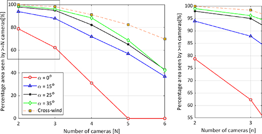
Figure 6. Inlet coverage from the multi-camera SPIV system at incidence and crosswind configuration. Right: zoom-in of the inlet coverage for two and three cameras.
Download figure:
Standard image High-resolution image2.3. Experimental conditions
The incidence measurements were performed at a freestream Mach number of 0.2 for a range of angles of attack between 25°–35°, with an increment of 1°. To simulate different intake operating points, the model exit mass flow was set equal to  and 100%, where
  is the maximum corrected mass flow of the suction system. Under the wind tunnel conditions, the Reynolds number Re for the incidence cases, defined in terms of the intake inner diameter and freestream velocity, was approximately equal to 1.1 ·106.
The crosswind measurements were performed primarily by varying the freestream velocity at a fixed value of mass flow through the intake, and secondarily by varying the intake mass flow at a fixed crosswind velocity. The crosswind velocity was varied in the range between 2 kts and 43 kts while the mass flow rate  was varied between 30% and 102% of
  . The intake performance in ground operation was investigated at a fixed representative vertical distance of h = 0.3Dhi (figure 1). The Reynolds number (
 ) for the crosswind cases varied between 0.3 × 10⁵ and 3.5 × 10⁵. To avoid early laminar separation, due to the low values of Re, boundary layer trips were used on the outer side of the intake surface. The complete test matrix of the experiments is provided in table 2, although only data for cases InW1, InW2 and XWS1 are addressed in the following sections of this paper.
Table 2. Test matrix for the incidence and crosswind configurations.
| Incidence | |||
|---|---|---|---|
| Dataset | AoA (α°) | Free stream Mach number, M∞ | Mass flow rate,  [%] [%] |
| InW1 | 25°–35° | 0.2 | 90 |
| InW2 | 25°–35° | 0.2 | 100 |
| Crosswind | |||
| Dataset | Crosswind velocity, V∞ [kts] | Mass flow rate,  [%] [%] | |
| XWS1 | 15 | 34–102 | |
| XWS2 | 15 | 102–34 | |
| XVS1 | 4–43 | 86 | |
| XVS2 | 3.5–30 | 100 | |
2.4. Data acquisition and processing
The PIV-data acquisition and processing was performed using the LaVision DaVis 11 software. The procedure was automated and interlinked with the wind tunnel operating software at DNW; this increased the productivity of the measurements and reduced the wind-on time for data acquisition. The measurements corresponding to the incidence sweep, which consisted of 60 data points (section 2.3) were completed in about 4 h.
Each data point measurement consisted of a sequence of 1000 double-frame images. Wind tunnel vibrations occurred during operation, which affected the camera images. To correct this, markers were placed on the outer surface of the inlet to facilitate the application of a shift and vibration correction algorithm (dots on the outer surface of the inlet in figure 7(a)). Image pre-processing was performed to remove the background light by normalising the pixel intensity with respect to the time-averaged value. After that, a minimum intensity over the subsequent 15 frames was subtracted from the images (figure 7(b)). In addition, the flow conditions in crosswind resulted in condensation of water around the ground vortex, which saturated the pixels in that region and inhibited the stereo reconstruction. To prevent spurious vectors, an algorithmic mask based on a threshold of pixel intensity was applied over this portion of the vortex. After this, the region of the image containing the particle images was extracted by the application of a geometric mask (figure 7(c)).
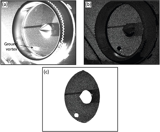
Figure 7. Raw image from a single camera corresponding to the crosswind configuration (a), image after pre-processing (b) and after application of geometric mask (c).
Download figure:
Standard image High-resolution imageThe image interrogation was performed using multi-pass cross-correlation with window refinement (Scarano and Reithmuller 2000). In the final iteration, windows of 48 × 48 px with Gaussian weighting were used with an overlap factor of 75%. The resultant vector spacing was 1.5 mm (corresponding to 0.006D, 0.6 vector mm−1), which resulted in 18 750 velocity vectors across the region of interest. To quantify the range of resolvable velocity scales, the dynamic velocity range (DVR, Adrian 1997) is determined as the ratio of the maximum measured velocity in the inlet plane and the standard deviation of the velocity distribution in the separated case. The details of the image processing parameters and estimates of the measurement dynamic range are summarised in table 3.
Table 3. PIV image processing parameters.
| Correlation algorithm | Multi-pass dual-frame cross-correlation | |
| Interrogation window | 48 × 48 px2 | |
| Overlap factor | 75% | |
| Vector pitch | Incidence | 1.5 mm |
| Crosswind | 1.5 mm | |
| Dynamic spatial range (DSR) | 30 | |
| Dynamic velocity range (DVR) | 100–125 | |
The average uncertainties in the particle displacement were calculated based on the correlation statistics described by Wieneke (2015). Figures 8(a) and (b) shows the uncertainties in mean velocity magnitude scaled by the mean axial velocity through the inlet. Figure 8(a) corresponds to the inlet at incidence where the flow is separated, and figure 8(b) to the crosswind case with the ground vortex and flow separation. The uncertainties in velocity are less than 2% in both configurations.

Figure 8. Contours of uncertainties in velocity magnitude normalised by the mean axial velocity through the inlet from the incidence (a) and crosswind (b). Contours of the normalized instantaneous axial velocity from the incidence (c) and crosswind (d).
Download figure:
Standard image High-resolution imageThe steady pressure measurements at the AIP were acquired over a period of 20 sec at an acquisition frequency of 625 Hz. The data were averaged over the duration of the PIV acquisition (for 1000 images, approximately 2 min).
For the current analysis, the PIV derived velocity maps are presented within the region between 0.3 R < r < 0.97 R, to ensure that no invalid measured data influence the postprocessing. Flow separation inside the intake was identified by means of the isoline of zero axial velocity for each snapshot, and the coordinates of the approximated centre of the separated region were calculated. The separation behaviour was further analysed considering the isentropic Mach number derived from the static pressure measurements around the intake wall:
For the crosswind cases where velocity measurements in the vortex core were available, the vortex core position at the PIV plane was identified for each instantaneous flow field by detecting the maximum value of the Q-criterion (Hunt et al 1988), defined as:
where  and
and  are the vorticity tensor and the strain rate tensor, respectively. Based on the definition, positive values of Q (i.e., Q > 0) are indicative of areas in the flow field where a vortex is present, provided that local static pressure is lower than the free-stream value. To avoid the interference of the vortical structures located inside the separated region, when present, and of the boundary layer region, only data within the region 135°—240° and r < 0.96 R was considered when performing the vortex core tracking.
3. Results
3.1. Intake at high-incidence
The contours of the time-averaged axial velocity, non-dimensionalised by the time-average area-average axial intake velocity, are reported in figure 9 and in figure 10, for the case at  = 90% and
  = 100%, respectively (cases InW1 and InW2 in table 2). The velocity fields correspond to a freestream Mach number of 0.2 and an incidence angle in the range 25°–35° for both intake operating conditions. The separation within the intake can be identified by the presence of a region of reversed flow, with negative axial velocity (figure 9(d)). From the observation of the flow fields reported in figures 9 and 10, starting from an attached flow condition (figures 9(a) and (a)), as the incidence angle increases, the flow inside the intake separates from the intake surface lip (figures 9(d) and 10(c)), generating a region of detached flow that increases in size with the angle of attack. Similar flow behaviour and flow topology, for which an intake exhibits lip separation due to high incidence angle, has been previously reported in several experimental works (Hodder 1981, Larkin and Schweiger 1992), which however relied only on conventional distortion measurement techniques, i.e. total pressure rakes.
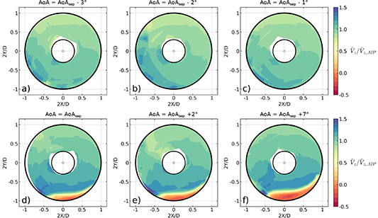
Figure 9. Variation of normalized time-average axial velocity across the range of incidence angles for case with M = 0.2 and  = 90% (InW1 in table 2).
Download figure:
Standard image High-resolution image
Figure 10. Variation of normalized time-average axial velocity across the range of incidence angles for case with M = 0.2 and  = 100% (InW2 in table 2).
Download figure:
Standard image High-resolution imageThe nature of this separation can be assessed by considering the peak isentropic Mach number variations with the angle of attack, as reported in figure 11, for the two intake mass flow settings, respectively. The isentropic Mach number (equation (1)) was calculated from the static pressure measurements around the intake surface at four different azimuthal coordinates on the bottom half of the intake surface. The angle at which the separation occurs for 90%  is 1° lower than for the case with 100%
  .
.
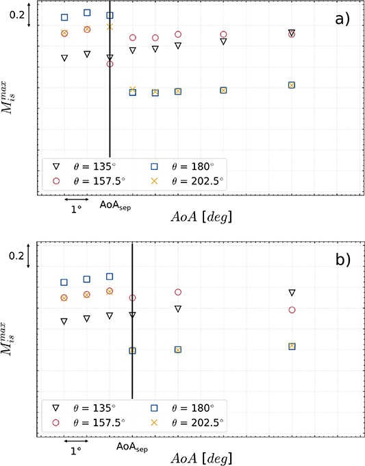
Figure 11. Peak isentropic Mach number variations with the angle of attack: (a) M = 0.2 and  = 100%; (b) M = 0.2 and
  = 90%. The black vertical lines indicate the separation angle.
Download figure:
Standard image High-resolution imageAs the angle of attack increases, the flow accelerates around the intake lip, resulting in a highly supersonic isentropic Mach number. At relatively low values of the incidence angle before the separation occurs, the flow is still attached to the intake surface, even though the boundary layer thickness becomes greater (figure 10(c)), indicating incipient flow separation. At the separation angle of attack, a shock is formed over the intake lip at 180° and 202.5°, causing the isentropic Mach number to drop to subsonic values and the flow separation.
3.2. Intake in crosswind with ground plane
The normalised axial velocity at the measurement plane with increasing mass flow rate is shown in figure 12 for a crosswind velocity of 15 kts and  between 34% to 102% (case XWS1 in table 2). As shown for the cases at high incidence, the separation within the intake can be identified by the presence of a region of reverse flow, with negative axial velocity. As the mass flow through the intake is increased, the intake flow goes from an initial separated condition (
 = 34%) to an attached condition (
 = 65%) and then separates again (
 = 94%). Due to the non-axisymmetric geometric features of the intake (scarf and droop angles) and the presence of the ground plane, the separated region is forced towards the top-half of the plane on the side exposed to the cross flow. As the corrected mass flow rate increases from 34% to 56%, the size of the distorted region decreases until the flow reattaches, at
  = 65%. As the
  is further increased from 85% to 94%, the flow separates again.
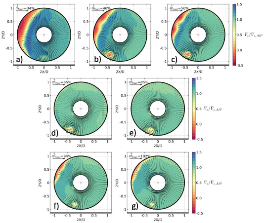
Figure 12. Variations of the normalized time-average axial velocity with increasing  (crosswind velocity 15 kts).
Download figure:
Standard image High-resolution imageSimilar flow behaviour for an intake in crosswind, for which two separation limits can be identified, has been previously reported in several experimental (Quemard et al
1996, Lecordix et al
1996) and computational studies (Colin et al
2007, Zhang 2021). For low values of the corrected mass flow  up to 56% of the maximum (figures 12(a)–(c), respectively) the separation is diffusion-driven. In these cases, the intake exhibits a wide area of reversed flow on the windward side and the distributions of the isentropic Mach number shown in figure 13, which provide information about the peak values, the position, and the extent of the separation, present a subsonic peak value. In these cases, there is a strong flow deceleration around the intake lip, highlighted by the presence of a plateau in the isentropic Mach number profiles in figure 13, causing the boundary layer to separate and form a large area of reversed flow. At high
  (from
(from  = 94% to
  = 102%, figures 12(f) and (g)), the separation is shock-induced, since the maximum isentropic Mach number for these cases, as seen in figure 13, is supersonic. The flow is strongly accelerated around the lip until it becomes locally supersonic. This generates a shockwave strong enough to cause the separation of the boundary layer. The presence of the shock wave can be identified in figure 13 by the presence of an abrupt drop in the isentropic Mach number. Between the two separation limits (
 = 65% and
  = 85%, figures 12(d) and (e)), the flow remains fully or mostly attached over the lip and the diffuser.

Figure 13. Isentropic Mach number profiles around the lip at four different azimuthal coordinates for case XWS1 (15 kts, increasing  ).
).
Download figure:
Standard image High-resolution imageIntake flows in crosswind are known to be characterised by a high level of unsteadiness due to the complex nature of the three-dimensional flow and the coexistence of flow separation and ingested vortex (Murphy and MacManus 2010, Wang and Gursul 2012). The instantaneous and time-averaged vortex core locations for the case at 15 kts with increasing (case XWS1 in table 2) are reported in figure 14, along with the probability of the vortex to occupy a specific location on the measurement plane.
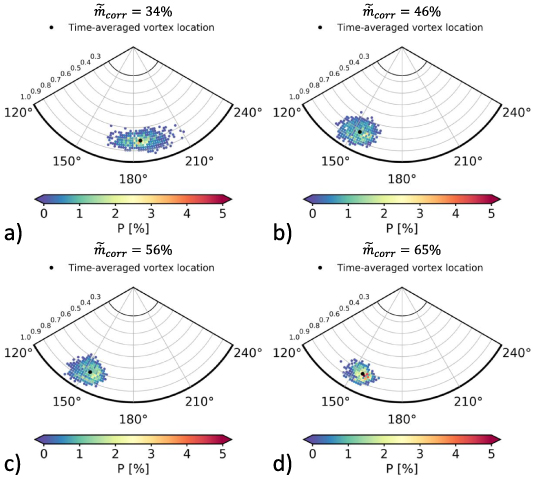
Figure 14. Instantaneous vortex location and probability P of the vortex to occupy a position on the measurement plane (symbols indicate the time-averaged location). Crosswind direction from left to right.
Download figure:
Standard image High-resolution imageIt can be observed that as the corrected mass flow is increased from 34% (figure 14(a)) to 65% (figure 14(d)) the ingested vortex is oscillating within a relatively narrower area around the time-average location, suggesting a decreasing level of unsteadiness. Moreover, at  = 34% (figure 14(a)), the area around which the vortex core location is oscillating exhibits an elongated elliptical shape compared to the one at
  = 65% (figure 14(d)), which presents a nearly circular shape. The difference in shape suggests that the vortex oscillation at
  = 34% is predominantly in the direction parallel to the crosswind velocity. Conversely, at
  = 65% the vortex oscillates in both directions, parallel and perpendicular to the cross flow, affecting a larger radial portion of the plane.
In terms of the lip separation, the instantaneous and time-averaged position of the centre of the separated area for three cases at 15 kts across a range of corrected mass flows  is reported in figure 15. The case with
  = 34% was found to be dominated by a diffusion driven separation, the case with
  = 65% was mostly attached and the case with
  = 102% showed a shock-induced separation. The centre of the separated region was defined as the centre of the circular sector enclosing the portion of the measurement plane where the reversed flow was present.

Figure 15. Instantaneous separated region centre and probability P of the separation centre at each location on the measurement plane (symbols indicate the time-averaged location). Crosswind direction from left to right.
Download figure:
Standard image High-resolution image
Based on the instantaneous positions of the centre of the separated area (figure 15), identified as the centre of the region with negative axial velocity, it can be observed that for the case with diffusion-driven separation ( = 34%, figure 15(a)), the radial extension of the separation is higher with respect to the cases characterised by shock-induced separation (
 =102%, figure 15(c)). For the case where diffusion-driven separation is present, the radial extent of the separated area covers almost 25% of the plane radius (figure 15(a)). On the other hand, for the case characterised by shock-induced separation (figure 15(c)), the separation is confined inside the outermost part of the measurement plane, near the outer surface of the intake, extending across a smaller part of the plane. It can also be noted that in the case at
  = 65% the time-average flow field is attached (figure 12(d)).
4. Conclusions
The current work was motivated by the established requirement to characterise the dynamic aspects of inlet flow distortion in aero-engine intake systems. Stereo PIV enables measurement of velocity data synchronously across a cross-flow plane with significantly higher spatial resolution compared to conventional pressure-based methods. Unsteady swirl distortion measurements in aero-engine intake ducts were previously reported at scaled, laboratory-based configurations but this current investigation is a further step ahead, demonstrating productionised swirl distortion measurements in an industrial environment. The paper addresses instantaneous inlet flow distortion measurements within a modern, through flow turbofan intake. using a stereo PIV technique. The measurements were performed using a novel stereo-PIV system comprising x6 sCMOS cameras with automated focus and Scheimpflug setup capability. The PIV cameras were integrated around the tunnel's working section and their lines of sight was optimised for optimum optical coverage of the measurement plane. An arrangement with two lasers illuminating the measurement plane from two different positions was used to mitigate the influence of the intake's nose cone in the plane illumination. The experiments were performed at the LST of the German-DNW, at a Reynolds number in the range 106–4 ·106 based on the inlet diameter which was approximately 250 mm at the fan-face. Swirl distortion measurements at a range of incidence and crosswind configurations were performed with a ground plane in place. The test matrix comprised a range of incidence angles between 25°–35° at two intake corrected mass flows as well as measurements across a range of crosswind speeds between 2 and 43 kts at a range of mass flows between 30% and 102% of  . The final achieved spatial resolution of the measured velocity fields was 1.5 × 1.5 mm2, which yielded approximately 18 000 three-component velocity vectors across the region of interest. This is two orders of magnitude higher than the resolution that a conventional pressure-based distortion rake system would provide. The incidence measurements, enabled the detailed characterisation of the cross-flow velocity field and the determination of the critical incidence angle on which separation occurs. The PIV data combined with the isentropic Mach number distributions along the intake lip, provided details about the nature of the separation mechanism and its impact on the dynamic non-uniformity of the flow delivered at the fan face. Similarly, for the cases with crosswind, the dynamic characteristics of the fan face flow field were quantified across the operating range. This included the unsteady behaviour of the ground vortex. Overall, the newly developed multicamera PIV system was found very efficient in acquiring high resolution PIV data across a representative range of incidence angles and crosswind conditions without manual calibration and re-adjustment of the optical setup. The developed capability enabled notably more effective use of the wind-on time in an industrial wind tunnel environment. The high-resolution data enabled the characterisation of the unsteady flow fields and swirl distortion metrics as well as their statistical analysis across a representative operating range. The acquired swirl maps constitute a major achievement and key enabler for future development of closely integrated engine-intake systems.
Acknowledgments
The project is conducted under Grant Agreement 864911 of the European Union's Horizon 2020 research and innovation program. Grant Agreement 864911 for Project NIFTI 'Non-Intrusive Flow distortion measurements within a Turbofan Intake'—H2020-CS2-CFP09-2018-02
Data availability statement
The data cannot be made publicly available upon publication due to confidentiality reasons.