

Abstract
We propose the use of a second surface mirror as a displacement plate-beamsplitter to provide significant simplification and cost reduction of time-of-flight anemometry (ToFA), without sacrificing precision and accuracy. These benefits are most pronounced for long-range applications. Our method's principle benefits are due to the few and simple components it requires as well as low sensitivity to both temperature effects and light source incoherence. We found that precise and accurate results are possible using a common consumer mirror as the main optical element and an inexpensive diode laser as the light source, which could broaden access to laser anemometry and make many industry applications economically feasible. The nature of the design also permits an increase in range for a given laser power since the method can utilize the entire optical area of the focusing lens/mirror independent of other design considerations and the cost of a flat second-surface mirror is usually negligible. To characterize the performance of this method, we develop a Cramer–Rao bound (CRB) for a general class of ToFA's with multiple Gaussian beams under signal-independent Gaussian white noise. For a given measurement volume, the lowest velocity uncertainty is achieved by creating a standard two-sheet geometry: power-matching the first two beams by adjusting the beamsplitter and blocking the rest of the beams is optimal. However, keeping the higher order beams permits determination of flow direction. Conditions to achieve beam power-matching are given. An anemometer is built using a diode laser with 12 mw 405 nm beam using a total of just three transmitting optical components. Our setup has an accuracy of 99.1%. The worst-case precision of 96.7% nearly achieves the CRB, although optimizing the setup more can lower the bound, and therefore allow increase in the performance by an order of magnitude or more.
Export citation and abstract BibTeX RIS

Original content from this work may be used under the terms of the Creative Commons Attribution 4.0 license. Any further distribution of this work must maintain attribution to the author(s) and the title of the work, journal citation and DOI.
1. Introduction
Laser anemometers are a good option for non-intrusive, spatial-temporally resolved measurements in fluid flows. Many different methods of laser anemometry exist, each with their own advantages and disadvantages, but they all have the same basic components and work on a similar principle. Excluding Doppler wind LIDAR and a few specialized techniques, laser anemometry infers the velocity of the fluid in the component normal to the beam pattern indirectly by measuring that velocity component of small tracer particle(s) that get carried passively by flow. To detect the velocity of a single particle it is necessary to first generate a precise beam pattern for the particle to pass through using a laser and various optical manipulations. The intensity of the scattered light from the particle will fluctuate in time according to the beam pattern, with the frequency of this fluctuation directly proportional to the particle velocity. The scattered light is collected, transduced, and then conditioned by a detector. Finally the signal is digitized and analyzed to give a single velocity reading. By the time the light is reflected by a particle it already encodes the velocity of the particle. As a result, much of the accuracy and repeatability of the sensor are tied up in generating a good beam pattern and ensuring its shape does not change over time.
Several beam patterns and pattern generation methods have proven successful. Time-of-flight anemometry (ToFA) is a common class of approaches that was first introduced to measure velocity from smaller aerosols, and closer to walls than the standard approach, laser Doppler anemometry (LDA), could achieve (Smart et al 1981, Albrecht et al 2003). Rather than generate an interference pattern by intersecting two beams as LDA does, ToFA generates fewer but more intense laser sheets or focal points at a given standoff distance from each other. This, in principle, also divorces the accuracy of ToFA from the laser's ability to act as a coherence standard since a change in wavelength need not change the beam spacing. The beam generation step is therefore even more crucial to overall performance of ToFA because the method of creating the beam profile will determine to what degree light coherence effects accuracy and repeatability. As a consequence, it determines what quality and type of laser and optics are needed. The exact parameters of the beam pattern itself will determine the repeatability of the sensor's measurements. Most ToFA methods generate two parallel beams using a Wollaston Prism and lens (Lading 1973, Wernet and Edwards 1986). These methods generally require careful alignment to ensure the beams are parallel and the correct distance apart. It can also only make one wavelength parallel at once, so it is not compatible with unstabilized diode lasers at large distances. Multiple detectors are needed if flow direction information is desired. Very small-scale ToFA and shear stress sensors have been achieved by micro-fabricating a diffractive optical element to produce a double-sheet pattern, but this is also wavelength dependent to first order and produces diverging rather than parallel sheets, so it is not effective at long range (Wilson et al 2000).
We propose a new method of generating the repeating pattern needed for ToFA that uses refraction rather than birefringence or diffraction. The method involves using a displacement plate-beamsplitter to generate multiple, identical, parallel output beams from a single input beam. Relatively high efficiencies are achieved at low cost by using a plate with a silvered rear surface, effectively making a second surface mirror. Since the method is refractive rather than diffractive or birefringent, as is the standard for ToFA, the effect of light incoherence only appears in higher-order considerations, when they appear at all. This is in contrast to more expensive methods based on a Wollaston prism, which are often more temperature and wavelength sensitive even at short range where loss of parallelism of the output beams is not a concern. This significantly reduces the requirements on the laser. Secondary reflections, commonly considered to be undesirable 'ghost beams' in the context of mirror optics are actually the working principle utilized in this method to generate shifted copies of the first reflection at the air-glass interface, and can be tuned by changing the angle of incidence to achieve a desired power content in these beams.
The existence of these 'ghost' beams is well known and used extensively in a beneficial manner for flat plate interference methods such as in etalons, the Lummer–Gehrcke interferometer, AR coatings, and the shear interferometer. However most designs using geometric optics, such as lenses, mirrors, and standard plate-beamsplitters, treat ghost beams as undesirable aberrations for their respective applications. A notable exception is the wedge beamsplitter where multiple internal reflections are used to generate multiple output beams, although the beams are not parallel and a reflective rear surface is not present (Beers 1974, Azzam 2007).
Herein we develop the theory of displacement plate-beamsplitter ToFA and subsequently demonstrate some of the system's desirable properties by characterizing a system using this design that utilizes inexpensive components. Theory is developed for beam power distribution, beam separation, and beam aberrations, required manufacturing tolerances, as well as the conditions required for matching the power content in the first two beams. Matching power in the first two beams is motivated in part by a Cramer–Rao bound (CRB) we develop. In its most general form, our CRB is applicable to any set of n identical and uniformly spaced Gaussian beams of arbitrary power with signal-independent Gaussian white noise. We also show that constructing the beam profile for ToFA using this method results in low sensitivity to temperature and light incoherence, meaning the method is compatible with a variety of low-cost light sources and applicable in extreme environments. A ToFA system using a consumer second-surface mirror and diode laser without temperature control or mode stabilization is constructed using this technique, and performance characteristics are determined.
2. Theory
To perform ToFA, two parallel and highly controlled beam profiles are usually desired. To generate this profile, we propose a new application of a standard optical element. The displacement plate-beamsplitter uses a second surface mirror at a large angle of incidence ( ) to generate a repeating beam pattern. This is possible due to partial external reflection off the glass surface, nearly complete reflection off the silvered surface, and multiple partial transmissions through the glass substrate. Specifically, the beamsplitter produces the first beam by specularly reflecting a portion of the power in the incident beam off of the first surface of the plate. The rest of the light gets refracted into the plate's interior where the light reflects specularly off of the plate's second surface. A fraction of this light power then gets refracted out of the plate so that it is parallel to the first generated beam. The rest of the light gets reflected, back towards the second surface again and the process continues until all of the light has either been transmitted or lost. Because of its inherently asymmetrical nature (a decaying tail in the overall amplitude of the higher order beams), this method produces a naturally existing feature for detecting reverse flows without the need for multiple detectors. If higher volumetric efficiency is desired, the higher order beams can be blocked (see discussion of the CRB for more on this). A diagram of the geometric optics of this optical element is shown in figure 1.
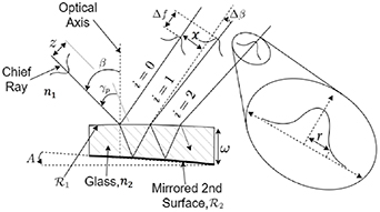
Figure 1. The optical setup for creation of multiple, parallel, identical-profile output beams from a single input beam at angle of incidence β. The separation between beams, x, is on the order of the flat plate's thickness, ω. The beam that gets reflected off of the glass is indexed as the i = 0 beam, and each sequential transmitted beam is indexed as  . The flat plate has an index of refraction n2 while the surrounding medium (usually air) has an index of refraction of n1. For calculation of aberrations due to manufacturing errors, a ray is allowed to be displaced by z from the chief ray of the input beam. Also, a small wedge angle A between the surfaces and large radii of curvature
  and
and  with common optical axis are allowed. These imperfections introduce slight alignment mismatch between the beams' chief rays,
  (both i and curv subscripts), here shown as a negative value. Also, even though the beamsplitter is nominally flat it modulates the focal depth of beams by the quantity
  (both s and p subscripts). For this reason it is necessary to consider rays that make an angle of γp
with the input chief ray (or, angle γs
out of plane, not shown). For uncertainty calculation purposes the beams are approximated as Gaussian, each with a
(both s and p subscripts). For this reason it is necessary to consider rays that make an angle of γp
with the input chief ray (or, angle γs
out of plane, not shown). For uncertainty calculation purposes the beams are approximated as Gaussian, each with a  radius, or half-thickness, of r in the thin axis of the laser sheets.
Download figure:
Standard image High-resolution imageTo properly design a ToFA system using this optical element, it is important to know the value of the standoff distance between each output beam, x, the level of aberration that occurs in the output beams, the allowable manufacturing tolerances, and the power in each beam for a given angle of incidence.
2.1. Beam separation
The first beam, which is reflected immediately, is denoted by the index i = 0. Each subsequent output beam, caused by partial tc  with the first transmitted beam being i = 1. The value of the separation distance between successive beams can be found through sequential applications of Snell's Law, and the result is well known. The plate thickness, ω, angle of incidence, β, and the ratio of material indices of refraction, ν, are related to the standoff distance, x, by, Wyant (1976)

By controlling the plate's thickness it is therefore possible to produce almost any beam separation at almost arbitrarily large or small distances from the beamsplitter because this equation holds true regardless of the diameter of the incoming beam, and it is relatively easy and inexpensive to produce large and flat glass plates. By making the incoming beam diameter large, possibly orders of magnitude greater than x, it is possible to keep the laser beam's numerical aperture large even for long range systems. As a result the beam spot size can be kept small relative to x, which produces higher signal to noise ratios and more precise measurements.
2.2. Beam aberrations
Since both optical surfaces are flat, if the beam is collimated each output beam's waveform is not distorted beyond distortions introduced by surface unevenness. The output beams are parallel to a very close approximation. This means the system's calibration is essentially the same regardless of depth. By utilizing the same lens for the laser and receiver (placed before the laser light reaches the beamsplitter), as is common for LDA and ToFA, the transmitter/receiver system becomes self-aligning.
However, one of the least attractive aspects of the displacement plate-beamsplitter in the context of ToFA is that if instead the beam is focused to a finite depth, this depth is altered for beams of order i > 0, and the quantity of this change depends on both the ray angle and the axis. This introduces defocusing, spherical aberration, astigmatism, and even coma. As a result, each beam will focus (in a slightly degraded manner) to its waist at a slightly different distance from the beamsplitter. Higher order beams will have a progressively degraded focus in the measurement volume as a result. Essentially, the system is self-aligning and focusing but the level of alignment and focus is not perfect and not independently tunable. Consider a ray of light that makes an angle of γs
with the chief ray from the laser diode (the ray at the axis of symmetry of the incoming beam) in a plane normal to the plane depicted in figure 1. The subscript s here relates to the plane in which the ray deviates from the chief ray and does not imply it is only relevant to a certain polarity of light. Due to symmetry, no coma is possible in this axis. However, as was already known at the time but analyzed in mathematical and numerical detail by Fried and Turner (1970), passage of this angled ray through the flat glass will alter the eventual location where this ray crosses the chief ray. The difference in location between beams of different orders ( , etc) where this ray crosses the chief ray as measured in the direction of propagation (using the location where the chief ray leaves the first surface as the reference point) can be described by,
where  is the difference in the index of the two beams being compared. The physical quantity this equation solves for is represented as
  in figure 1. Since this is a non-trivial but even function of the ray angle, spherical aberration is introduced. The reason this equation differs somewhat from Fried and Turner (1970) is because the beam is folded and placed on an angle.
Now consider a ray of light that makes an angle of γp , from above, with the chief ray (ie, it has a higher incidence angle) in the plane depicted by figure 1. For this ray, the difference in focal distance between it and the focal distance of the two beams (again in the direction of propagation) is given by,
This equation represents the same physical quantity as  , so it too is represented as
  in figure 1. However, because it comes from an angular deviation that is orthogonal to the one that causes
  , its value is different. Since this equation is not even, coma is introduced. Since it is not identical to equation (2), astigmatism is introduced. As γs
and γp
tend to zero, the spherical aberration and coma disappear, but the defocus and astigmatism remain. Assuming
, its value is different. Since this equation is not even, coma is introduced. Since it is not identical to equation (2), astigmatism is introduced. As γs
and γp
tend to zero, the spherical aberration and coma disappear, but the defocus and astigmatism remain. Assuming  is small for all rays in the beam relative to the depth of focus, the beams will focus to a diffraction limited sheet at the same depth. The depth of focus for a Gaussian beam can be written in terms of the laser's wavelength, λ, and the half apex angle, Θ
Comparison of b and  is critical for designing a system with sharp focus. The signal strength for laser anemometry depends directly on the beam's power density, and measurement uncertainty also decreases when the beams are thin compared to their separation. These equations imply the displacement plate-beamsplitter performs best when the numerical aperture is kept small enough to avoid aberrations but not so small that the beam waist is undesirably large.
2.3. Tolerances
The theory developed thus-far assumes a plate with perfect parallelism, perfect flatness, and immaculate surface quality is used. Real flat plates have none of these properties. The multiple reflections and two refractions experienced by higher order beams as well as the high angle of incidence present in this beamsplitter will amplify any imperfections in construction. This makes the allowable tolerance on the plate quite small. Luckily the methods available for producing flat plates, and especially flat surfaces, are among the most foundational and well refined in the fields of optics, metrology, and various industries. It is possible to obtain flat glass plates with extremely small tolerances that suffice to allow it to be used as a displacement plate-beamsplitter.
The required parallelism tolerance is the most difficult to achieve both because the effect of a small wedge angle is greatly amplified at large distances, and because it is more difficult to align two planes to each other than it is to produce a single pristine plane. Using the results of Beers (1974), we can derive a formula for the difference in angle between the 0th and ith beams,  . This quantity, represented as
  , is shown in figure 1. Note that in this figure the angle shown is a negative value. For a beamsplitter with wedge angle A, one can re-derive a result first produced but not published by Beers (1974),
This formula shows high angles of incidence greatly increase the sensitivity to A. Consider the case of s-polar light, where β is tuned such that the power contained in the i = 0 and i = 1 beams are the same, ν is not approximately 1, and  . With these assumptions a convenient approximation for
  exists:

More information on beam power matching and the definition of ξ are given in section 2.6. Intuitively this equation results in the conclusion that for practical designs  . If the beams converge or diverge too much their separation at the depth of the intended measurement volume will be too great. To achieve
  at 1 m measurement distance,
  should be 25 arcseconds at most to avoid the chance of the beams crossing in the measurement volume. At greater range, for smaller ω or higher β, if predictable calibration is desired (especially at multiple depths), or if more beams are kept, the requirement becomes even more strict. Optical flats and optical windows can be obtained with parallelism of <5 arcseconds without difficulty whereas lower parallelism tolerances come at an increasing premium. The parallelism of float glass varies significantly from batch to batch and even across a given pane, however we did not find it difficult to obtain float glass mirrors with parallelism in the vicinity of 1 arcsecond.
Surface flatness effects the beamsplitter's performance in three primary ways. Firstly each beam gets re-focused by the curvature of the beamsplitter's two faces. Secondly, beams of different orders interact in a slightly different way with the beamsplitter's slight curvature and thus they are not parallel to each other anymore. Finally, if the diameter of the beam at the displacement plate-beamsplitter is comparable to the distance over which the curvature changes, the complex surface unevenness profile will show up as further aberrations that will appear in the focused beams. To make analysis tractable it is convenient to assume the beamsplitter is locally spherical with radius  on the first surface and radius
  on the second surface (concave down is positive). It is also convenient to use the best-fit parabola to mathematically approximate this spherical curvature. It is assumed that the axis of these surfaces are aligned, forming an optical axis, and that the chief ray strikes the first surface at the optical axis. Assuming the input beam is collimated, one can track the position and angle of a ray through the beamsplitter if the ray has a displacement of z from the chief ray (see figure 1). For the i = 0 beam, a reflection off of the first surface is experienced, so this is just a classic parabolic reflector (the math is fairly simple in this case, and both focus and aberration have been fully studied). For instance, for a parabolic reflector one can derive an equation for the intersection depth of a ray with the chief ray (assuming the reflector's height variation can be ignored and assuming surface slope is small),
When β is small this reduces to the classic result for the focal length of a spherical mirror or best-fit parabolic mirror,  . Increasing β increases the focusing power of any slight curvature in the first surface as well as producing progressively greater coma.
The i = 1 beam is produced from refraction off of the first curved surface, reflection off of the second surface, and then refraction again off of the first surface. By tracing a ray through this path it is possible to obtain an expression for the angle between the reflected chief ray for the i = 0 beam (reflected at angle β) and the i = 1 transmitted ray (that started z above the chief ray). The angle between higher order beams can also be determined but the formulas become unwieldy. Using some trigonometry and using the same small slope and height assumptions as before, the angle difference  is found to be,
The intermediate variable κ represents the angle the ray makes to the optical axis after entry into the glass. The variable d1 represents the distance from the optical axis to where the ray hits the second surface. The variable d2 is the difference in distance (from the optical axis) between where the ray of interest reached the first surface from within the glass and where it first reached the second surface. The quantity  represents the loss in parallelism due to imperfect flatness in the beamsplitter. Figure 1 shows
  as
as  . It is important to note that much less parallelism error is introduced if
  (about 5 arcseconds if
  , regardless of ν, for β of roughly 75∘) than if
  (about 100 arcseconds if
  , regardless of ν, for β of roughly 75∘). Due to the way it is manufactured, float glass tends to have curvature of the same sign on both surfaces whereas for optical flats this is not likely. Even though optical flats have vastly superior flatness, the types of manufacturing errors made by float glass are less costly so the performance gap is smaller than expected. The depth where the ray of interest crosses the chief ray in the i = 1 beam (measured along this chief ray from where it left the beamsplitter) can be found using,
To a good approximation, the beam re-focusing effect described by f1 is caused exclusively by reflections. This is true for beams of all orders, not just the first beam. The reason is because for beams i > 0 the beam encounters exactly two refractions that almost exactly cancel the focal effect of each other (one when entering the glass and one when leaving it). If  then behavior of a given ray is almost the same for the i = 0 and i = 1 beams (
 ). As a result, it is a good approximation to assume
  and so any re-focusing effect caused by surface curvature will be eliminated almost entirely during initial alignment. This holds true even for fairly large z. Therefore, the only relevant and potentially significant error introduced by identical (first and second surface) local surface curvature in a displacement plate-beamsplitter is classical parabolic reflector coma. If the beam diameter at the displacement plate-beamsplitter is a significant fraction of the length scale over which the radius of curvature in the glass changes, complex surface-specific beam aberrations will occur. The magnitude of these more complex aberrations can be approximated using equations (7)–(9) as a starting point.
While surface quality can be an important optical consideration, we expect it to rarely be critical for this application despite the high angle of incidence and multiple reflections. The reason is both because the beam is not focused on the displacement plate-beamsplitter (so the power density is low, and imperfections are not focused into the measurement volume), and because it is more difficult to achieve acceptable levels of parallelism in the plates than acceptable levels of surface quality through polishing.
Considering  and
and  are generally more important than
  in determining performance, properly sourced and inspected float glass should be competitive with precision ground optical flats in terms of performance despite their significantly lower cost. More generally this analysis shows that tolerancing issues should not be prohibitive even with designs that take advantage of the longer ranges this method enables.
2.4. Beam power
The power in the  beam, Pi
, can be found by applying the Fresnel power equations to each reflection or transmission, accounting for the reflectivity of the second surface, Rm
. When this is done, equation (10) results. Similar calculations have been performed by others for wedge beamsplitters, (Beers 1974)
beam, Pi
, can be found by applying the Fresnel power equations to each reflection or transmission, accounting for the reflectivity of the second surface, Rm
. When this is done, equation (10) results. Similar calculations have been performed by others for wedge beamsplitters, (Beers 1974)
where  is the total power incident onto the displacement plate-beamsplitter. The analysis is greatly simplified by the fact that the fraction of light transmitted on each internal reflection at a glass-air interface, R, is equal to the fraction of light initially reflected off of the glass at the air-glass interface (Beers 1974). The Fresnel equations in the p and s-polar cases are used to find this fraction, R,
Note that the beamsplitter produces degenerate outputs for excessively large and excessively small angles of incidence since,
2.5. CRB
Under the assumption that the main source of noise is Gaussian and signal-independent (ie shot noise from unwanted background light entering the detector, or thermal noise), it is possible to use a CRB to find the minimum possible uncertainty in measured velocity resulting from a single particle passing through n Gaussian beams spaced x apart, each with  beam radius r and power Pi
. The relative 1 standard deviation precision in measurement velocity V is bounded by,
beam radius r and power Pi
. The relative 1 standard deviation precision in measurement velocity V is bounded by,
where  is the ratio between beam width and beam separation, and
  is the signal to noise ratio. The value for
  can be determined by summing the amplitudes of the Gaussian peaks observed in a return signal or it can be predicted from first principles using the laser beam's power output, the particle scattering parameters, and the definition given in the
  , and when
  (ie, equation (10) is not used) (Fischer et al
2010). The general case for η, which allows for any number of beams of any arbitrary power level so long as they have the same width and they are Gaussian is,
(ie, equation (10) is not used) (Fischer et al
2010). The general case for η, which allows for any number of beams of any arbitrary power level so long as they have the same width and they are Gaussian is,
Important properties of η are that it is invariant to changes in laser power, invariant to spatial shifts, and invariant to spatial scale. This means η is an intrinsic quantity related to the geometry of the beam pattern itself. Under the assumptions leading to equation (10) (ie, our setup), and in the limit of infinite numbers of beams (which would occur if the measurement volume were infinitely wide), η can be expressed in terms of just Rm
and the ratio of the power in the first transmitted beam to the reflected beam,  ,
,

The expression utilizes the definition  where R is fully specified by Rm
and
where R is fully specified by Rm
and  . In fact it can be shown that
  . The expression for RL
follows from its definition and equation (10). A graph of
. The expression for RL
follows from its definition and equation (10). A graph of  as a function of
  for
for  is given in figure 2.

Figure 2. Signal efficiency  as a function of the ratio of power in the first two beams,
  , with
  (−). The value of
  is given for the scenario where the measurement volume is nominally x, 2 x, and
  wide (corresponding to sensing only the first two, three, and all beams). Also shown is
  for a standard two-spot setup under the assumption of zero power loss, which is given by Fischer et al for equal beam powers and given in general from equation (14). by assuming
  (
( ). Notice the maximum of
  for our configuration, where the measurement volume's width greatly exceeds x, occurs at
  , while the maximum for a two-spot setup occurs at
  as is expected.
Download figure:
Standard image High-resolution imageAs illustrated in figure 2, putting more of the laser's energy in the first beam results in the greatest signal efficiency, however the cost of doing so is higher incidence angles are needed to achieve this state. Therefore the sensor will experience greater sensitivity to changes in angle (ie from vibration or setup error) as well as greater difficulty detecting the other peaks in the presence of other forms of noise. The performance degrades both when  and
and  , as expected, since in either case almost all of the energy goes into a single output beam.
Compared to two-spot or two-sheet ToFA, our method has greater efficiency for all  , although this is because the higher order beams of our method increase the effective sampling volume: equation (15) assumes an unbounded measurement volume by considering an infinite number of beams. Often only the first few beams (at most three or four) are needed to achieve similar performance to that given in equation (15). This is shown by the
  curves in figure 2 where only three of the generated beams are in the measurement volume: performance is similar to when all of the beams are in the measurement volume. Regardless of how many beams are kept in the measurement volume, when considering any number of beams truncated at n > 2, for a given x, the measurement volume of our method exceeds that of two-spot or two-sheet ToFA. Therefore, for a given volume two-spot ToFA can be more power efficient if the beam splitting method is highly efficient, but only by at most
  if the second surface for our method is highly reflective (see equation (19) and subsequent discussion). Actually this means that our method is up to
  efficient at producing a two-spot beam by blocking off or otherwise ignoring the higher order beams, which is lower than most two-spot methods but not greatly so. Note that the
  curve when two beams are in the measurement volume is not quite identical to the two-spot curve, even if re-scaled, because the two-spot curve does not include a power loss model that changes with
  .
.
Matching the power in the first two beams often strikes a good balance between maximizing η and achieving reasonable signal profiles and incidence angles. It also allows detection of reverse flow if the third beam is kept. Indeed, figure 2 shows  achieves nearly optimal values of η regardless of how many beams are kept in the measurement volume. If just two beams are kept, the performance is very close to optimal. We now discuss various aspects of this special configuration both due to its theoretical advantages (especially if only the first two or even three beams are kept) and to illustrate various aspects of the beam profile in general.
2.6. Beam matching
It is possible to tune the angle of incidence, β, in order to match the power of the first reflection and the first transmission beams ( ). In fact, any power ratio between the i = 0 and i = 1 beams is possible in most cases. The tuning angle required to match power in the first two beams can be calculated algebraically. This is done by setting
  using equation (10), substituting equation (11) for R, and solving for β. The result is,
Notice that the beam power matching equations depend only on two variables: the index of refraction ratio at the beamsplitter's first surface, and the reflectivity of the second surface. These equations are plotted in figure 3. Notice that for the s-polar orientation there always exists a value of ν such that a desired matching angle β is achieved, while for p-polar light the matching angle achieves a well-defined extremum at just above ν = 1 and just below  . If the beam spacing is strongly dependent on β, the system is more difficult to align and more susceptible to vibration. Also if
  is high relative to b, the level of defocusing between beams in the measurement volume will be significant. Since
  is smaller for β close to 45∘ and
  is smaller near this angle too, the s-polar orientation has significant theoretical advantages, especially for high index materials (but not exceeding ν ≈ 3).
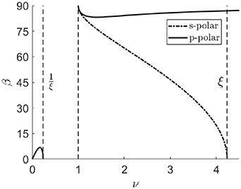
Figure 3. The beam-matching value of incidence angle β as a function of index of refraction ratio ν, with mirror reflectivity  . Notice how a minimum angle of incidence occurs for p-polar light at ν ≈ 1.4 but no such minimum exists for s-polar light.
Download figure:
Standard image High-resolution imageIt is not always possible to match the power of the two beams as indicated by the fact that these equations do not always return a real number. This is the case if the argument of the square root is negative or if the argument of the inverse cosine exceeds 1. For s-polar light, beam matching is only possible if  and
and  , which implies
  and
and  . For positive indices of refraction, the combination of these two requirements can be expressed as,


For p-polar light and positive indexes of refraction, for the same reason, it is only possible to match beam powers in the domain,
Therefore in the p-polar case there is a small region of index of refraction space where beam matching is possible and also  . This suggests a second potential configuration for beam splitting. The configuration is more compact than the conventional one since the angle of incidence is small. However it is only possible to achieve in special circumstances such as with infrared light and a Germanium-air interface since
  . See figure 4 for a depiction of both the conventional and second configuration.

Figure 4. A depiction of how the displacement plate-beamsplitter can be configured with the laser to generate a desired output beam pattern. Configuration 1 is the conventional setup. It uses a large angle of incidence. This works for both p-polar and s-polar light. Configuration 2 uses a slight angle of incidence and a transition from high index to low index rather than from low index to high index, making it a possibility for fiber lasers. Configuration 2 is only compatible with p-polar light and is only feasible in special circumstances.
Download figure:
Standard image High-resolution imageThe amount of light contained in the first two beams when the beams are forced to have the same power is independent of polarization as well as ν. The rest of the light is absorbed, or goes into the periphery beams. When the beams are tuned to this angle, at each glass-air interface, the fraction of light reflected is given by the solution of  for R. This comes directly from setting
  in equation (10). The solution for R under this constraint, denoted by
  , is
, is
The other root obtained is non-physical. Notice only one independent variable is present, Rm
. The maximum amount of light contained in the first two beams, if they match powers, occurs when  . According to equation (19), this means the maximum power in the first two beams when they are matched is
  . Substituting
  for R into equation (10), it follows immediately that after the first two beams the light contained in each successive beam decreases geometrically as follows

Again the only independent variable in equation (20) is Rm
. Since this variable is generally close to 1, the power fraction in each beam is essentially universal under the condition that  . The beam powers for
  are shown in figure 5.

Figure 5. The power fraction in each beam as described by equation (20) where the mirror reflectivity, Rm
, is 1 (the height of each black vertical line represents the power fraction in a given beam). Cumulative power, defined as the sum of the power in each beam along with those preceding it  , is also shown as black circles.
Download figure:
Standard image High-resolution image2.7. Temperature sensitivity
A laser anemometer's temperature sensitivity comes from differences in the Doppler shift sensitivity in LDA (usually equivalent to a fringe spacing difference) or changes to the beam separation for standard ToFA methods (Kitchen et al 2003). We show theoretically that the temperature sensitivity is negligible in our setup using an unstabilized Sanyo 405 nm laser diode and soda-lime glass displacement plate-beamsplitter with 20∘ C room temperature. All of the properties used for the calculations in this section are given in table 1.
Table 1. Laser and beamsplitter properties used to calculate temperature and coherence errors.
| Parameter | Value |
|---|---|
| Rm | 0.9 |
| ν | 1.54 Rubin (1985) |
| ω | 2.8 mm |

| 1 nm |

| 1 nm |

|
 Ashby (2013) Ashby (2013) |
| λ | 405 nm |

| 0.06 nm
|

|
 nm−1 Rubin (1985) nm−1 Rubin (1985) |

|
 Jewell (1991) Jewell (1991) |
| β | 82.9∘ |
The sensor's temperature dependence comes from a combination of changes to the index of refraction induced by lasing wavelength changes, glass expansion, and index of refraction changes with temperature. The values provided in table 1 are used to approximate the change in index of refraction with respect to a small change in temperature,
This means  . This result can be used in conjunction with equation (1) to find the change in separation distance with respect to a small temperature change,
For our setup this means  . The partial derivatives of x can be obtained by differentiating equation (1). Close to our linearization temperature, the temperature induced error rate in velocity readings is,
For our setup a value of  is found. The proposed method is therefore essentially temperature insensitive because a 100 ∘C temperature change will cause only a 0.1% measurement error.
2.8. Incoherence sensitivity
The effect of the laser's incoherence on x is very important when using an unstabilized laser diode without temperature control because most diode lasers exhibit poor coherence properties on their own. Since our method uses geometric optics only, temporal coherence is not a factor. Non-ideal spectral coherence on the other hand can reduce both accuracy and precision. It could also potentially limit how small x can be made because dispersion broadening of the beam spacing could broaden the beams into each other for sufficiently small x (note however that dispersion does not change the degree to which the output beams are parallel). The change in beam separation for a given wavelength drift, which is also the peak width increase for a given spectral bandwidth (due to dispersion), is given as follows,
Since the change in beam spacing is directly proportional to  , low dispersion is beneficial for this method. However, we have already stated the benefits of high ν when using an s-polar configuration, but high index of refraction materials generally have low Abbe numbers. The choice of plate material is a tradeoff. For our setup a value of
  is found. For a 1nm wavelength drift or a 1 nm FWHM spectral bandwidth (both are typical for a diode laser), the corresponding wavelength fluctuation or beam width increase is
  of x. As a comparison, two beam LDA has a fringe spacing relation of
  where θ is the angle between the two beams, so
  and this is true regardless of the angle between the beams (in reality there are also other reasons to stabilize a diode laser for LDA) (Albrecht et al
2003). Beam width broadened and beam separation are therefore affected very little by dispersion resulting from the laser's lack of spectral coherence in our setup despite using a glass with moderate dispersion properties. Hence, even for unstabilized diode lasers we recommend optimizing ν rather than the Abbe number. Non-ideal spatial coherence limits how small the focal point can be and thus how small the measurement volume can be, but otherwise does not effect accuracy or precision directly. Since this method does not put strong restrictions on the light source's coherence it may even be possible to use non-lasing sources so long as their spectral radiance is sufficient to achieve good signal to noise ratios.
and this is true regardless of the angle between the beams (in reality there are also other reasons to stabilize a diode laser for LDA) (Albrecht et al
2003). Beam width broadened and beam separation are therefore affected very little by dispersion resulting from the laser's lack of spectral coherence in our setup despite using a glass with moderate dispersion properties. Hence, even for unstabilized diode lasers we recommend optimizing ν rather than the Abbe number. Non-ideal spatial coherence limits how small the focal point can be and thus how small the measurement volume can be, but otherwise does not effect accuracy or precision directly. Since this method does not put strong restrictions on the light source's coherence it may even be possible to use non-lasing sources so long as their spectral radiance is sufficient to achieve good signal to noise ratios.
3. Methods
For a proof of concept experiment, a Sanyo 405 nm laser diode was chosen due to its relatively Gaussian beam shape and low cost. The single-mode beam shape allows for precise multi-sheet pattern to be produced with just a focusing lens to focus the diode's expanding beam, a 50 mm focal length plano-convex cylindrical lens to create the laser sheet, and the displacement plate-beamsplitter to generate the repeating beam pattern of laser sheets from the single sheet (see figure 6). The chosen angle of incidence was 82.9∘, and the displacement plate-beamsplitter was cut from a 2.8 mm thick glass-front mirror. The mirror was held at the chosen angle using a 3D printed mount. The laser diode has a measured power output of 12 mw. The beam profile as defined by a Gaussian fit has parameters  , r = 0.0828 mm (the diffraction limit is 0.03 mm), and δ = 6.62. In our setup with a cylindrical lens and circular beam, it is the orientation of the lens rather than the polarization of the diode's beam that is aligned with the long axis of the laser sheet. For this reason and because we did not have precise control of the diode's orientation in its heat sink, we did not utilize equation (16) to ensure
  . Figure 7 shows the beam profile used in the experiments.
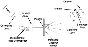
Figure 6. The experimental setup. The forward-scatter configuration allows a translucent pinhole to be used to simulate a particle passing through the beams (the detection configuration is not a focus of the experiment). Depiction not to scale.
Download figure:
Standard image High-resolution image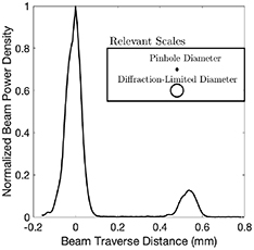
Figure 7. Beam profile resulting from the optical setup, with two other relevant lengths (in the box) for scale. The profile was extracted from the pinwheel experiments by ensemble averaging the data. The pinhole size is clearly much smaller than the beam diameter. Notice that the beam powers do not match, which is a result of the 3D printed mount being printed for a polarity that was not observed in the experiment due to the difficult in controlling the diode's orientation during setup. This reduced η relative to a power-matched profile.
Download figure:
Standard image High-resolution imageThe detector is a side view R3896 Hamamatsu PMT. A 10 nm FWHM bandpass chromatic filter and lens-pinhole spatial filter are used to reduce noise. The 1/10th intensity detection volume is 10 mm3 and the distance to the detection volume from the detector is 258 mm. The distance to the detection volume from the beamsplitter is 287 mm. The relatively large detection standoff distance was chosen in order to determine if the laser sheet profile and alignments can be controlled precisely at these distances with this new method, and because this ensures the defocusing and aberrations discussed in section 2.2 would not be an issue. In our setup  , so b = 16 mm. At the same time,
  mm for
  with 0.2% variability in this value of
  being possible for values of γp
corresponding to rays at the edge of the beam (mostly caused by coma). Therefore the lag between beam focusing is about 3× smaller than the depth of focus.
being possible for values of γp
corresponding to rays at the edge of the beam (mostly caused by coma). Therefore the lag between beam focusing is about 3× smaller than the depth of focus.
The performance of the sensor was determined using a pinwheel as the velocity standard (ITTC 2008). A  pinhole (with translucent white material placed behind it to spread the transmission beyond that induced by diffraction) was placed at a known distance from the center of rotation of the wheel, thus allowing laser light to pass through to the detector once per revolution. The pinwheel standard has a velocity uncertainty based on a 95% confidence interval (CI) of 0.2%; the uncertainty sources are 0.1% from angular velocity, and 0.1% from radial position of the pinhole. This was determined based on the measurement tolerance of the pinhole location as well as the statistics of the fluctuations in rotation frequency of the pinwheel measured across the range of speeds used for testing;
  to
to  (95% CI).
The algorithm used for extracting velocity from the raw intensity return is a standard autocorrelation method with sub-sampling-rate resolution. The sub-sampling-rate resolution is achieved by fitting a parabola to the first prominent autocorrelation peak with non-zero shift. Points within 1/4th the distance to the closest prominent autocorrelation minimum is used to fit the parabola.
4. Results and discussion
The calibration test shows the laser anemometer has a maximum-deviation accuracy of 99.1%, and a maximum one-standard-deviation precision of 96.7% when using a single particle/pinhole pass for measurement. The calibration test results are plotted in figure 8, from which it can be determined that the beam separation distance is 0.551 mm. Equation (1) predicts  . This is less discrepancy than the precision with which ω was measured, which implies
  is on the order of arcseconds (see equation (5)). The fact that the relation is not a direct proportion indicates the existence of a slight bias either in the algorithm, the pinhole reference velocity, or in the circuit. The beam profile from the experiments are shown in figure 7. Note how the beams are of similar widths, but their profiles are not quite Gaussian and not quite identical due to spatial noise along the direction of propagation. This is typical of an unstabilized diode laser.

Figure 8. The calibration test results. The pinhole's velocity is on the vertical axis, and the measured autocorrelation shift is on the horizontal axis. Note that the slope of the linear regression of these points (−) is the previously unknown beam spacing.
Download figure:
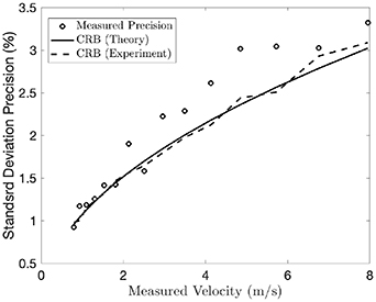
Standard image High-resolution imageA graph of the precision at each speed tested alongside the Cramer–Rao lower bound given in equation (13) using equation (15) is shown in figure 9. In this figure the theoretical CRB uses the values of  , δ, and
  found at the lowest velocity along with the
  dependence of
  for the calculations, while the experimental CRB curve uses the values found in the data at each velocity. Notice that equation (13) bounds the precision from below quite tightly. The remainder of the precision deficit is likely a combination of the non-Gaussian nature of the beam profiles, unaccounted-for noise sources, and the fact that our auto-correlation peak-detection algorithm is neither a minimum variance unbiased estimator, nor even a maximum likelihood estimator of velocity (Lading 1983, Lading and Edwards 1993). On the other hand the bias detected in the calibration curve indicates that precision is somewhat artificially deflated. Therefore the gap between the CRB, which in its common form is for unbiased estimators, and the achievable unbiased precision with our setup may be larger than figure 9 indicates. Further improvements to the accuracy and precision can be achieved by increasing δ and by making
  . ToFA systems often use δ as large as 95, which would improve the precision, and possibly accuracy, by an order of magnitude (Smart et al
1981). Changing
. ToFA systems often use δ as large as 95, which would improve the precision, and possibly accuracy, by an order of magnitude (Smart et al
1981). Changing  can improve the light utilization efficiency from
  to as much as
  .
.
Figure 9. The one standard deviation precision of the anemometer at each speed measured, with the Cramer–Rao lower bound (CRB) given in equation (13) plotted as well. The CRB as calculated from the parameters found at the lowest velocity and then inferred at other velocities (−) is plotted alongside the CRB as calculated from the parameters found at each velocity (−−). Despite the algorithm's non-optimality, the CRB is essentially achieved. This may be in part because the algorithm and the setup have slight bias, and because the beam is sharper than a Gaussian.
Download figure:
Standard image High-resolution image
5. Conclusions
We proposed a ToFA system that uses a displacement plat-beamsplitter to generate multiple light sheet profiles from a single input light sheet that can be configured to detect reverse flows in a natural way without needing multiple detectors. Our experimental setup used just three optical elements and a low cost laser diode on the transmission side in a non-optimal geometry, but achieved 99.1% accuracy with 96.7% worst-case precision. We developed a CRB for the sensor's precision, as well as for a more general class of ToFA's, and the sensor we constructed nearly achieves this bound. Our experiments in conjunction with the CRB indicate that with a larger beam separation ratio and equal distribution of power between the first two beams, the method could be useful for precision sensing applications without increasing cost; even when used for two-spot anemometry, the power efficiency can be as high as 76.4%, and both the bias and random errors can be reduced by an order of magnitude simply by changing δ and  .
.
At the same time, the nature of the beamsplitter means the input beam is copied and displaced without altering its shape, so all other optics can be placed before it. This allows, for instance, the beam separation to be much greater than the diameter of the beam as it passes through the beamsplitter. In long-range applications this is helpful because the entire focusing optical area can be utilized, and the numerical aperture of the focusing optics (and thus the beam waist thickness) and beam separation can be controlled independent of each-other and the range without incurring large cost. It also makes a fully self-aligning setup straightforward to produce. The setup is especially well suited for harsh environments where our method's insensitivity to environmental factors such as temperature, and possibly even vibration, are important. The downside is that various optical aberrations are introduced, the largest relevant one being that beams of different orders focus to a point at different depths. This is unimportant for long-range applications where the focusing lens' numerical aperture is small, however it limits large numerical aperture applications.
The main benefits to our method are its intrinsic simplicity and ease of construction, as well as its usability with low cost diode lasers and other light sources (so long as they have high radiance and moderately narrow spectra) as well as low cost optics, especially at long range. As the cost of laser diodes and photodetectors continue to fall, we expect the cost of a short or moderate range ToFA system based on our method to be determined by the cost of the chromatic band-pass filter, if one is used, or otherwise the sensor housing or data collection and processing device, depending on the specific engineering requirements and economies of scale involved. This would open access to laser anemometry to a wider group of scientists and engineers who cannot otherwise afford laser anemometers, and possibly facilitate uses outside of fundamental research such as feedback systems or even consumer handheld devices.
Acknowledgments
We would like to thank Luke Rumbaugh and William Jemison for their insightful discussions and support, and Erik Bollt and Morteza Gharib for their comments on the manuscript.
The experimental results presented herein were obtained in a facility at Clarkson University whereas some of the theory and data analysis was done afterwards while under the support of the NSF GRFP at Caltech.
Data availability statement
The data cannot be made publicly available upon publication because they are not available in a format that is sufficiently accessible or reusable by other researchers. The data that support the findings of this study are available upon reasonable request from the authors.
Funding
This material is based upon work supported in part by the National Science Foundation Graduate Research Fellowship under Grant No. DGE-1745 301. Any opinions, findings, and conclusions or recommendations expressed in this material are those of the author(s) and do not necessarily reflect the views of the National Science Foundation.
Disclosures
A provisional patent filing based on part of the work presented here is in-process.
Appendix
The derivation given here is for the Fischer information of the parameter vector ![$\theta = [V, P_0,r,t_0]$](https://content.cld.iop.org/journals/0957-0233/34/9/095301/revision3/mstacd657ieqn136.gif) , as well as the CRB for V. This derivation is a natural extension of the two-spot anemometer result given by Fischer et al (2010). The major difference is that here the bound is valid for any beam pattern composed of multiple Gaussian peaks so long as they have the same width and the same separation, while the two-spot result of Fischer et al (2010) is specific to the standard two-spot configuration. Our bound on velocity measurement variance agrees with theirs in the special case that they consider when n = 2 beams of equal power are used.
, as well as the CRB for V. This derivation is a natural extension of the two-spot anemometer result given by Fischer et al (2010). The major difference is that here the bound is valid for any beam pattern composed of multiple Gaussian peaks so long as they have the same width and the same separation, while the two-spot result of Fischer et al (2010) is specific to the standard two-spot configuration. Our bound on velocity measurement variance agrees with theirs in the special case that they consider when n = 2 beams of equal power are used.
We assume that n beams are in the measurement volume. We also assume that the power received by the detector from a particle at position y in the 0th beam is  so that the area under the Gaussian beam profile for the 0th beam is
  . The parameter
  represents the fraction of beam energy that is captured by the detector for a particle located at position y. This function changes for each particle, but is approximately the same as a given particle moves through each of the n beams. A detector such as a photo-multiplier tube is used to take M equally time-spaced samples from the photon detection frequency function,
where  is known apriori but P0 is not, and
  is the energy contained in one photon. The index i is the beam number, where i = 0 is the first reflection, i = 1 is the second, etc. The detector samples this distribution discretely over time interval
  , indexed by k, giving the discrete function
  . This function measures the number of photons captured in each sample of length
  rather than the photon detection rate.
The number of photons detected is corrupted by the existence of signal-independent additive Guassian white noise, Nk
. That is, at every sample point, the probability density function of Nk
is  . As a result of the noise introduced by Nk
, the actual sampled value is
. As a result of the noise introduced by Nk
, the actual sampled value is  rather than
  . The log-likelihood function is,
The log-likelihood summand is  . The Fischer information matrix is the negative expectation taken over the data of the log-likelihood Hessian,
  ;
; ![$\mathbf{F}\equiv -\mathbb{E}[\mathbf{H}]$](https://content.cld.iop.org/journals/0957-0233/34/9/095301/revision3/mstacd657ieqn150.gif) . Regularity was confirmed for n = 2 by Fischer et al (2010), so it follows that it holds for any finite n as well. Since
. Regularity was confirmed for n = 2 by Fischer et al (2010), so it follows that it holds for any finite n as well. Since  is deterministic and also the only function of the parameters, the Fischer information matrix is
where ![$\mathbb{E}\left[\frac{\partial^2 l_{ik}(\theta)}{\partial \overline{f}_{ki}^2}\right] = \frac{1}{\tau^2}$](https://content.cld.iop.org/journals/0957-0233/34/9/095301/revision3/mstacd657ieqn152.gif) . If
. If  then the tails of the beams have little overlap, so it is sufficient to approximate the problem by assuming the samples are taken each from their respective nearest peak,
 ![$\overline{f}_{ki} = \frac{\Delta t P_0 Y R_i}{E_\mathrm {photon}\sqrt{2\pi}r}\exp{\left[-\frac{2V^2(k\Delta t-t_0-ix/V)^2}{r^2}\right]}$](https://content.cld.iop.org/journals/0957-0233/34/9/095301/revision3/mstacd657ieqn154.gif) , rather than taken from the entire underlying profile fk
. Furthermore, if in addition
, rather than taken from the entire underlying profile fk
. Furthermore, if in addition  , the sum in k can be replaced with an integral on
  , and this can be evaluated exactly.
The definition  was used to shorten the expression, and only the upper half of the matrix is presented because it is symmetric.
According to the multi-variate CRB without priors, the covariance matrix K is bounded from below, in the sense of positive semi-definiteness, by the inverse of the Fischer information

The variance bound of interest is the one on element K44, although the other elements can be quite useful since they bound the other parameter estimate variances. A fundamental property of positive semi-definiteness is that if a matrix is positive semi-definite, each of its diagonal entries must be as well. Therefore  , (Cover and Thomas 2005)


The dimensionless parameter δ represents the ratio of the beam separation to the beam width. The dimensionless parameter  is a function of only the allocation of power to each of the n beams in the measurement volume, and is therefore a measure of the beam utilization efficiency. Note that
  is invariant to spatial shifts, ie
  , as it should be. The dimensionless parameter
  represents the ratio of detected signal to detector noise (both in terms of photons counted). The expression for
  given allows the signal to noise ratio to be determined before setting up the experiment by utilizing the expected parameters of the laser beam and flow velocity. The appearance of the flow velocity in the signal to noise ratio comes from the fact that faster moving particles return less intense signals because they are in the measurement volume for less time. The grouping of terms in the expression for
  shows that it is also possible to read the signal to noise ratio directly off of a return signal by calculating the standard deviation of the noise (in units of volts rather than photons), and determining the signal level (also in volts) by taking the peak height of the 0th beam's signal.
In many cases it is more convenient to consider signal to noise ratio in terms of the total laser power rather than the power in the first beam. In this case, we can define the following new parameters,
In terms of these variables, the relative uncertainty in measured flow velocity is a simple manipulation of equation (30),
For the special case of a displacement plate-beamsplitter, it is known that  , and
, and  for i > 0 (equation (10)), so,
Further specializing to the case where  and using
  , it is possible to produce a closed form expression. The following infinite sum identities are useful: for
  ,
,  ,
,  ,
,  . The result is,
It is possible to re-express this equation by replacing R with  . To do so, use equation (10) and solve the quadratic equation resulting from
  :
:  (the positive root is not relevant).