

Abstract
One of the most significant and growing research fields in mechanical and civil engineering is structural reliability analysis (SRA). A reliable and precise SRA usually has to deal with complicated and numerically expensive problems. Artificial intelligence-based, and specifically, Deep learning-based (DL) methods, have been applied to the SRA problems to reduce the computational cost and to improve the accuracy of reliability estimation as well. This article reviews the recent advances in using DL models in SRA problems. The review includes the most common categories of DL-based methods used in SRA. More specifically, the application of supervised methods, unsupervised methods, and hybrid DL methods in SRA are explained. In this paper, the supervised methods for SRA are categorized as multi-layer perceptron, convolutional neural networks, recurrent neural networks, long short-term memory, Bidirectional LSTM and gated recurrent units. For the unsupervised methods, we have investigated methods such as generative adversarial network, autoencoders, self-organizing map, restricted Boltzmann machine, and deep belief network. We have made a comprehensive survey of these methods in SRA. Aiming towards an efficient SRA, DL-based methods applied for approximating the limit state function with first/second order reliability methods, Monte Carlo simulation (MCS), or MCS with importance sampling. Accordingly, the current paper focuses on the structure of different DL-based models and the applications of each DL method in various SRA problems. This survey helps researchers in mechanical and civil engineering, especially those who are engaged with structural and reliability analysis or dealing with quality assurance problems.
Export citation and abstract BibTeX RIS

Original content from this work may be used under the terms of the Creative Commons Attribution 4.0 license. Any further distribution of this work must maintain attribution to the author(s) and the title of the work, journal citation and DOI.
Abbreviations
| AE | Autoencoders |
| AI | Artificial Intelligence |
| AL | Active Learning |
| AL | Active Learning |
| ANN | Artificial Neural Network |
| Bi-LSTM | Bidirectional-LSTM |
| CAE | Contractive Autoencoder |
| CNN | Convolutional Neural Networks |
| DAE | Denoising Autoencoder |
| DBN | Deep Belief Network |
| DL | Deep Learning |
| DOE | Design of Experiment |
| DRL | Deep Reinforcement Learning |
| DTL | Deep Transfer Learning |
| FEM | Finite Element Method |
| FORM | First Order Reliability Method |
| FOSM | First Order Second Moment |
| GAN | Generative Adversarial Network |
| GRU | Gated recurrent unitsUnits |
| LSF | Limit State Function |
| LSTM | Long short-term memory |
| MCMC | Markov Chain Monte Carlo |
| MCS | Monte Carlo Simulation |
| MLP | Multi-Layer Perceptron |
| MLP | Multi-Layer Perceptron |
| MLS | Moving Least Square |
| MPP | Most Probable Point |
| MSE | Minimum Square Error |
| NLO | Nonlinear Oscillator |
| NN | Neural Network |
| NPF | Nonlinear Performance Function |
| Probability Density Function | |
| PF | Performance Function |
| PoF | Probability of Failure |
| RBF | Radial Basis Function |
| RBM | Restricted Boltzmann Machine |
| RNN | Recurrent Neural Networks |
| RSM | Response Surface Method |
| SAE | Sparse Autoencoder |
| SOM | Self-Organizing Map |
| SORM | Second Order Reliability Method |
| SRA | Structural Reliability Analysis |
| SVM | Support Vector Machine |
| VAE | Variational Autoencoder |
1. Introduction
The term 'reliability' was primarily taken as repeatability. A system was assumed reliable if the same test results were achieved after repetition of the experiment. Thus far, this definition has been enhanced and stated as: Reliability is the 'probability of a system or component performing its intended functions under specified operating conditions for a specified period of time' [1]. Under the stated definition, different SRA methods have been developed so far. Regarding the definition of reliability, SRA methods use the lifetime probability of structural response to find when it crosses the safe domain of operation (or, in other words, failure criteria) to calculate the probability of failure or reliability. Generally, the lifetime probability of structural response can be calculated through sampling methods. The initial samples can come from analytical calculations, FEM [2], or experimental measurements [3]. The experimental data represents the structure's response and it can include different parameters such as the structural strain that is measured using a strain gauge [3], or the vibration data that is measured using accelerometers [3]. Accordingly, the accuracy of the SRA is highly dependent on the sampling or the response measurement methods. Therefore, advanced and precise measurement techniques are necessary to achieve accurate experimental data and reduce uncertainties [4].
Although advanced and improved measurement techniques can reduce the uncertainties and improve the accuracy of condition monitoring data, there is still a need for methods to quantify the remaining uncertainties and take them into account, especially for high-accuracy and reliable systems, such as nuclear powerplants and transportation system [5]. As the reliability analysis deals with different uncertainties, in such cases, SRA can play a constructive role in taking the uncertainties into account and improving structural safety in different situations [6]. Considering modelling or measurement uncertainties, statistics appear in various reliability analysis activities, such as sampling and DOEs. An accurate reliability estimation method considering various uncertainties from measurements to modelling can play a significant role in improving the design and performance of mechanical and structural systems [7–9]. An effective SRA can also help with the justification of design for different working conditions based on design and performance requirements [10, 11]. As the system becomes more complicated and safety is also of concern, an accurate SRA can become a very time-consuming task [5, 12], which makes it more critical to apply efficient novel methods for the SRA. With the growth of computational methods, the application of statistical theories in recognition and prediction of patterns and machine learning (ML) methods were established. Afshari et al have presented a review of ML-based SRA methods in [13]. But recently, DL has quickly developed as a leading technique of ML and captured outstanding attention from scholars worldwide [14]. DL can be considered a special kind of ML, which is upgraded to deal with more complex problems automatically with fewer human inputs. This paper reviews the applications of DL-based methods for SRA to investigate the justification of varying DL-based approaches for a practical inclusive SRA.
Before reviewing the applications of DL methods in SRA, it is helpful to understand the meaning of the terms reliability and structural reliability. Reliability is defined as 'the probability of a system or component, performing its intended functions under specified operating conditions for a specified period of time' [1]. As stated in [13], calculating the failure probability that is defined below in equation (1) is a key activity in most SRA problems,
where  is the failure probability,
 ![${f_{{\boldsymbol{x}}\left( t \right)}}\left[ {{\boldsymbol{x}}\left( t \right)} \right]$](https://content.cld.iop.org/journals/0957-0233/34/7/072001/revision2/mstacc602ieqn2.gif) is the joint PDF of the random variables vector,
is the joint PDF of the random variables vector,  , and
, and  is the PF being used for reliability analysis, which is also recognized as LSF [13]. There are well-established methods to solve common types of reliability equations. For instance, Given the equation
  , methods based on Taylor expansion, such as FORM or SORM have been used to solve equation (1) analytically. However, they need some detailed knowledge about the LSF, which usually comes with a high computational cost. Another well-known SRA approach is MCS, which is also a computationally expensive method [15]. Accordingly, in need of more computationally efficient algorithms, especially for complex systems, surrogate modelling is introduced to the existing SRA methods for approximating the LSF in a more effective way [13].
Surrogate models can be considered differentiable estimations of the LSFs [1]. In recent decades, substantial progress in different ML methods has helped SRA methods with finding surrogate models of the PF or the LSF or even the reliability index [13]. However, ML-based techniques have challenges with compromising the accuracy and computational time of the SRA. In such cases, new methods like DL-based techniques have received increasing attention. DL-based SRA methods follow a pretty similar structure to ML-based methods but with slightly different algorithms. A significant requirement for DL-based SRA methods is the higher required training sample size as compared to ML-based methods. Therefore, researchers have also tried to apply DL-based sampling methods to decrease the number of training samples while keeping the accuracy to improve the model's efficiency. Accordingly, DL techniques are becoming increasingly popular, especially for nonlinear or high-dimensional problems where computational efficiency is a challenge [13, 16–18].
DL-based methods usually consist of a set of connected neurons, ordered in several layers between inputs and outputs, helping them learn complex functions more easily than a single neuron or layer can. Each layer extracts some features from its inputs, and each subsequent layer extracts features from the previous layer's outputs. In this sense, DL pulls high-level latent features from lower-level features and data [16]. The idea of the hierarchy of extracted features is a basis for the superiority of DL-based methods. The depth of a DL method refers to the number of hidden layers between the network's inputs and outputs. Thus far, DL-based methods have been primarily used in problems with high-dimensional data in which the system's dimension is a significant barrier. For example, in SRA problems, ML problems become exceedingly difficult when the data dimensions are too high. This phenomenon is known as the curse of dimensionality. The reason behind that challenge is that the sum of the variables increases exponentially as the number of dimensions increases in nonlinear or high-dimensional problems.
Furthermore, when equipped with convolutional layers, DL-based methods are highly influential in handling high-dimensional data sources. Figure 1 roughly shows the performance comparison of DL and ML modelling considering the number of samples required for solving the SRA problem. This comparison shows why DL-based methods in SRA have received increasing attention for more complex problems when more samples are needed to maintain an accurate SRA for complex structures.

Figure 1. Performance comparison between DL-based and ML-based algorithms for SRA versus the number of required samples to maintain an accurate SRA.
Download figure:
Standard image High-resolution imageUnderstanding when a DL-based method works well for an SRA problem is an important task. In many SRA applications, we may need to deal with rare events' probability, which means a limited amount of training data is available. Furthermore, the general modelling approach (such as linear, nonlinear, nonparametric, etc) needs to be selected deliberately, which can make challenges in using DL-based methods. Moreover, finding accurately labelled data may become challenging via experiments or analysis. In such cases, DL-based algorithms seem to be the most practical approaches for the SRA. In figure 2, a general DL-based algorithm workflow to solve SRA problems has been shown, which involves three steps: understanding and preprocessing the data, building and training the DL model, and validation and interpretation. Unlike the classical ML modelling, we see more automation in step 2 of the DL model [19].

Figure 2. A DL-based algorithm workflow to solve SRA problems, which includes three stages.
Download figure:
Standard image High-resolution imageIn this paper, we go through different DL techniques used in SRA literature. We also present a classification of DL techniques based on how they are used to solve various SRA problems. However, before exploring the details of the DL techniques, it is helpful to review the main types of learning tasks that are (i) supervised: a method that uses labelled training data, and (ii) unsupervised: a method that analyses unlabelled datasets, (iii) semi-supervised: a combination of supervised and unsupervised methods. Therefore, to present our classification, we divide DL-based methods generally into three major categories: deep networks for supervised, unsupervised and hybrid learning, as shown in figure 3. In this paper, we introduce those techniques that have been used to practically solve SRA problems. We are also covering some novel works that can also potentially be classified as ML-based techniques that are not covered in our previous publication on ML-based methods for SRA problems [13].

Figure 3. Deep learning-based SRA methods can be divided into three major categories.
Download figure:
Standard image High-resolution imageThe remaining part of this paper is structured as follows: Supervised DL-based methods and their application for SRA are reviewed in section 2. Section 3 presents a review of the SRA methods using unsupervised methods. Section 4 surveys the hybrid DL-based methods for SRA, followed by a discussion and methods comparison in section 5. Finally, conclusions are given in section 6.
2. Supervised methods
The labelled data are commonly achievable through experiments or numerical/analytical analysis in SRA literature. Hence, supervised algorithms appear to be practical approaches for many SRA problems. These methods can be categorized into classification and regression methods. Classification approaches are mainly used for discrete output data, and Regression algorithms mostly deal with continuous output data [20]. Figure 4 shows the supervised learning process [13], where  represents the function or distribution that will be modelled. It should be noted that
  is usually taken as the LSF or the PF in the SRA problems. The inputs vector (features vector) is represented by
  and
and  is the quantity of features, and
  is the estimated output. The set of input–output pairs, designated by
  , is obtained from the probability distribution of inputs,
  . The it
h sample data pair is denoted by the superscript
. The it
h sample data pair is denoted by the superscript  , and H is a set of all probable models, and the final hypothesis,
  H, is designated by the ML algorithm. The ML algorithm uses an optimization technique to choose the optimum values of parameters '
 ' regarding cost functions, such as least square error or maximum likelihood. The optimization procedure is known as 'model training' in the ML literature. The estimation of
  at each operating point,
  , is the model's output shown by
  . The selection of the explained parameters depends on various factors, such as the number of features in the input, the size and dimension of the data, and prior knowledge about the input/output distributions. For example, the computational cost for some ML algorithms significantly rises with the number of features. Accordingly, ML algorithms should be justified to maintain accuracy and efficiency, resulting in different approaches. MLP, CNN, LSTM, and GRU are the most used supervised methods in the SRA studies, and they are presented separately in subsections below.

Figure 4. Supervised learning schematic process.
Download figure:
Standard image High-resolution image2.1. MLP
MLP can be used for SRA in various engineering fields, such as civil, mechanical, and aerospace engineering. The MLP can be used as a surrogate model for time-consuming and computationally expensive simulation-based methods, such as MCS, for evaluating the reliability of structures. In SRA, the MLP can be trained on a set of input-output pairs generated from simulation-based methods to learn the relationship between input variables (e.g. loads, material properties, geometries) and output variables (e.g. stresses, strains, displacements). The trained MLP can then be used to predict the output variables for new input variables, enabling efficient and fast evaluation of the structural reliability. The use of MLP in SRA has several advantages over traditional simulation-based methods, including reduced computational cost, faster convergence, and improved accuracy. However, it is important to ensure that the MLP is trained using a sufficiently large and representative dataset to avoid overfitting and to validate the model's accuracy before using it for real-world applications.
An MLP is an entirely connected ANN, as shown in figure 5. A typical N-layer MLP. Weights connect the nodes in two contiguous layers. The output of a node is defined as follows:

Figure 5. A typical N-layer MLP.
Download figure:
Standard image High-resolution imagewhere l is the number of layers, d is the number of nodes,  is the weight,
  is the bias, and
  is an activation function.
As pointed out by Schmidhuber [14], it is not clear in the literature at which level shallow learning ends and DL begins. An attempt to define shallow and deep NNs is presented in [21], where it is said that deep architectures are composed of multiple levels of nonlinear operations. In this paper, we use simpler criteria that shallow networks are those with just a single hidden layer, while deep NNs are those with more than one hidden layer [22, 23].
A large number of applications of MLP in the field of structural reliability have been presented in the literature, as can be seen in our previous review paper [13]. However, most employed shallow NNs with just one hidden layer [24–26]. Many recent publications have shown that deep NNs usually outperform shallow ones [22, 27]. Deep NN has a strong capacity for approximation relationship learning between two data spaces. With more hidden layers, deep NNs can handle more complex problems or multiple interactions between parameters [28].
The number of hidden layers in deep MLP is not limited. It depends on the architecture or complexity of the investigated structure. It has been shown that using two hidden layers is generally sufficient to solve a complex SRA problem [29, 30]. For MLP-based SRA, the input layer may consist of the structure properties [31], design variables [23], and operational conditions [32]. In the output layer, the value of LSF is generally chosen as the output [22, 33]. The PF [30], or the reliability index [34] is also reported as the output.
Combinations of MLP with FORM, SORM, and MCS are commonly used strategies for SRA. Section 1.1.1 summarizes the literature on MLP-based FORM or SORM. MLP-based MCS are presented in section 1.1.2.
2.1.1. MLP-based FORM or SORM.
The basic idea underlying FORM or SORM is to estimate the LSF by its first or second-order Taylor expansion at the design point. In the direct FORM and SORM, the derivatives usually require complex calculations. When it comes to MLP in combination with FORM or SORM, the responses and their derivatives can be easily obtained by the chain partial differentiation rule [13]. It has achieved great success in the shallow NNs for SRA [35]. Deep NNs-based FORM and SORM are also very popular for SRA in recent years.
To reduce the time cost of calculating the structural response of complex systems, Lehky and Somodikova utilized MLP with two hidden layers to approximate the original LSF [36]. First, a stratified Latin hypercube sampling simulation method is used to select the training set properly. Then, the MLP is updated close to the failure region to increase the accuracy. Then FORM is used to evaluate the reliability. The method is employed in the reliability assessment of three bridge structures, showing that the technique is efficient whether the LSF is defined in explicit or implicit form. Malekzadeh and Daei proposed a hybrid FORM-sampling simulation method for efficient reliability evaluation [31]. MLP approximates the LSF using two hidden layers. It can overcome the obstacles in the differentiation of LSF, especially when the LSF is nonlinear and non-differentiable. The design point is determined step-by-step with the IS and limiting the STD of the sampling density function. The proposed method can assess structural reliability with few random samples.
In addition, Wen et al adopted MLP with four hidden layers to approximate the joint PDF of the pipeline's reliability [33]. They investigated the influence of the ordering of training samples on pipelines' reliability prediction results. An optimization of MLP was performed to find the best approximated joint PDF. Then, the reliability was assessed by direct integration. Their method showed high efficiency and accuracy in comparison with non-optimized MLP models and the MCS method.
2.1.2. MLP-based MCS.
MLP-based MCS is most popularly used in MLP-based SRA [37–40]. Jha and Li [41] introduced the high dimensional model representation into MLP to approximate implicit LSFs in SRA. The computational results show their method not only yields accurate results but also reduces its computational efforts compared to direct MCS. Lee and Lee [34] developed an efficient sampling-based inverse reliability analysis method combining MCS. MLP with two hidden layers is used to train the relationship between the realization of the performance distribution and the corresponding true percentile value. Thus it can be applied to any type of PF. A dimension reduction method is proposed to eliminate the limitation of training data size. A comparative study using various mathematical examples shows that the method can obtain a more accurate percentile value estimation. Li et al [42] presented a novel hierarchical neural hybrid method to efficiently compute failure probabilities of challenging high-dimensional problems. Multi-fidelity surrogates are constructed based on two-hidden layer MLP with different levels of layers, so expensive high-fidelity surrogates are adapted only when the parameters are in the suspicious domain. Nie et al proposed a framework for fatigue-induced SRA of steel bridges based on four-hidden layer MLP and MCS [32]. The traffic-characteristic and non-traffic-characteristic parameters are taken as the inputs of the MLP, while the value of LSF is chosen as the output. The effects of truck weight limits and cracks are considered. It can quickly predict fatigue failure for a steel bridge under truck weight limits.
Recently, AL has received extensive consideration. It can be applied to train the surrogate models with a limited number of initial experimental samples and a small number of newly added experimental points that approach the LSF surface iteratively [23]. Gomes used deep MLP with AL for LSF approximation in SRA [22]. The experimental design is enriched by the k-means clustering method and a learning function related to the misclassification probability. The comparison results show that the deep NNs with more than one hidden layer required fewer calls to the LSF and achieved better accuracy than the shallow ones. Xiang et al adopted the weighted sampling method to select experimental points located in the interface of the safety and failure MC populations [43]. Uniformly distributed sample points can be selected from the MC population, and the selected points get close to the LSS iteratively. In each iteration, MLP with two hidden layers is updated to predict the value of LSF. The proposed method can achieve high accuracy with fewer calls of the LSF compared with AK-MCS and IS. Bao et al developed an adaptive subset searching-based MLP to solve the problem of optimal local sampling in AL-based methods [23]. The MLP with two hidden layers is utilized to approximate the LSF. An adaptive construction method is developed to regulate the size of each hidden layer. The method can obtain high-accuracy predictions with fewer experimental points when calculating the failure probability. Lieu et al built an approximate global model of PF based on MLP with two hidden layers [30]. They proposed an adaptive learning method by adding important points on the boundary of LSF and their surrounding zones. A threshold is adapted to switch from a globally predicting model to a local one for the approximation of LSF by eradicating previously used unimportant and noise points. By comparison with AK-MCS, IS + ANN, et al, the paradigm is more effective and precise for the failure probability estimation with only a fewer number of PF calls. Table 1 summarizes the reviewed studies of the application of MLP in SRA problems.
Table 1. Summary of applications of MLP (more than two layers) in SRA problems.
| Reliability method | Sampling method | Hidden layers | Input | Output | Case study | Reference, Year |
|---|---|---|---|---|---|---|
| MCS | Active learning with weighted sampling | 2 | Structure properties, load | LSF | Series system including four branches, a non-linear oscillator, a cable-stayed bridge | [43], 2020 |
| MCS | Active learning with important subsets | 2 | Structure properties, load | LSF | Modified series system, a cable-stayed bridge | [23], 2021 |
| MCS | Active learning with a learning function | 2 | Structure properties, load | Performance function | Truss structures | [30], 2022 |
| MCS | Kernel density estimation method | 2 | Morphing parameters | Reliability index | 6D arm model | [34], 2022 |
| MCS | Orthogonal design | 6 | Firmness coefficient, traction speed, and cutting depth | LSF | Structure of shearer cutting part | [37], 2022 |
| MCS | Random | 2 | Random variables in partial differential equations | LSF | High-dimensional problems | [42], 2019 |
| MCS | Random | 2 | Structure properties, rotor speed | LSF | A rotating disk, a ten-bar truss structure | [41], 2017 |
| MCS | Active learning | 2,3,4,5 | Structure properties, load | LSF | 23-bar truss structure, series system with four branches, two-Dimensional Truss Structure | [22], 2020 |
| MCS | Random | — | Size parameters, load, tensile strength | LSF | Plexiglas plates with holes | [38], 2020 |
| MCS | Random and the orthogonal design | 4 | Traffic-characteristic parameters and non-traffic-characteristic parameters | LSF | Steel bridges | [32], 2022 |
| MCS | Experimental data | 3 | Concrete strength, lateral pressure | LSF | Concrete under triaxial compression | [40], 2019 |
| Direct integration | LHS | 4 | Structure properties, defect properties | LSF | Pipelines | [33], 2019 |
| FORM | LHS | 2 | Strength properties, load | LSF | A pitched-roof frame, a concrete slab bridge | [36], 2017 |
| FORM | Random | 2 | Structure properties, load | LSF | Truss structures, two-floor two-span concrete structure | [31], 2020 |
Although deep NNs perform well, shallow ones are effective and sufficiently accurate in many fields. They are still prevalent and have been successfully used recently [44–46]. The papers published after 2019 are included in this review though one hidden layer is used.
The integrated use of MLP with FORM/SORM/MCS is widely adopted. Jia and Wu proposed an efficient SRA method combining MLP and Laplace asymptotic integral [25]. MLP with an AL function is employed to approximate the LSF near the target design point. The AL function proceeds through the optimization formulation without a candidate sample population. The superiority of the proposed method is validated by comparing it with existing Kriging and ANN-based methods. Pradeep et al analysed the reliability of the embedded depth of sheet pile based on a hybrid MLP with Various optimization techniques [47]. They used the MLP to forecast the embedment depth of a cantilever sheet pile wall considering the uncertainties of soil properties. And FORM was used to predict the reliability. The results show that MLP with teaching–learning-based optimization and MLP with imperialist competitive Algorithm performed best during the training and testing. Tawfik et al developed an MLP-Based SORM for the laminated composite plates in free vibration [48]. The MLP is used to obtain the fundamental frequency of composite plates by considering the uncertainties of geometric and material properties. Hence, the time-consuming finite element (FE) algorithm in the stochastic analysis is replaced. Therefore, the proposed method is much faster compared with direct MCS. Besides, it can take into consideration of the complex ply thickness uncertainty. Mathew et al proposed an adaptive Importance Sampling-based MLP model for variable stiffness composite laminates, which leveraged the advantages of both the MLP-based SORM and Importance sampling [49]. MLP is trained to obtain the value of LSF with hybrid uncertainties. The importance sampling density is centred around the MPP estimated iteratively by SORM. The method is in close agreement with ANN-based MCS and takes half the time. Aiming to solve the complex and expensive damage analysis of composite structures, Azizian and Almeida constructed an efficient FE-based reliability method with MLP and central composite design [26]. MLP is used to approximate the burst failure pressure with uncertainties in the physical and mechanical properties. A strategy is presented using the Plackett–Burman method to choose the main uncertainty sources so that the computational burden in non-deterministic analyses can be alleviated. The results show that their method works efficiently and more accurately than the commonly used response surface methodology. Ren et al used the ensemble of surrogates with ANN and Kriging to solve the challenge of reliability evaluation with limited knowledge of the LSF [50]. Then merits of both two models can be captured. The goodness of each surrogate model is measured locally. The surrogate models are updated by two proposed AL approaches. Compared with the single surrogate model with AL methods (e.g. AK-MCS), the proposed method is more effective in assessing the reliability of high-dimension and rare event problems.
Wakjira et al [51] proposed models for predicting the shear capacity of beams, considering critical variables. The so-called extreme gradient boosting model showed the highest prediction ability among the ML models they tested. In their study, SRA is performed to calibrate the resistance reduction factors to achieve target reliability for the proposed model. They used an MLP-based model for predicting the shear capacity of strengthened RC beams, considering all critical variables. The results showed that their proposed MLP-based models could be successfully used to predict the shear capacity of such strengthened beams. Wakjira et al [52], also presented a data-driven approach to determine beams' load and flexural capacities. Among their studied MLP-based models, the xgBoost is the most accurate, with the highest coefficient of determination. A comparison made in their study of the performance of various existing analytical models revealed the superior robustness and accuracy of their proposed model. Table 2 summarizes different studies using MLP with one hidden layer in SRA.
Table 2. Summary of applications of MLP with one hidden layer in SRA problems.
| Reliability method | Sampling method | Input | Output | Case study | Reference, Year |
|---|---|---|---|---|---|
| FORM | Random | Soil properties | Performance function | Sheet pile walls | [47], 2022 |
| FORM | — | Structure properties, load | Performance function | A spatial structure | [46], 2021 |
| SORM | Random | Geometric and material properties | Performance function | Laminated composite plates | [48], 2018 |
| SORM | Active learning | Structure properties, load | LSF | An aero-engine turbine disk, a ring-stiffened cylinder | [25], 2022 |
| MCS | Central composite design | Physical and mechanical properties of composite | Performance function | Composite structures | [26], 2022 |
| Important sampling | LHS | Geometric and material properties | LSF | Variable stiffness Composite laminate | [49], 2020 |
| MCS | Random | Geometry sizes, material properties and loads | Performance function | A head pressure shell | [45], 2021 |
| MCS | — | Geometry parameters, resistance parameters | LSF | Steel four-bolt unstiffened extended end-plate | [44], 2021 |
| MCS | Active learning | Structure properties, load | LSF | A cantilever tube, an offshore wind turbine jacket | [50], 2022 |
2.2. CNN
CNN have been commonly adopted for a wide range of engineering problems, especially in vision-based tools (image segmentation and classification) [53]. Recently, CNNs were successfully modified to be used for SRA, especially when there are uncertainties in physical properties [53–55]. Recently, CNNs have been mainly adopted in civil and mechanical engineering as a method for structural health monitoring, such as detecting surface cracks and structural faults [56, 57]. The logic behind the CNN-based SRA is that CNNs can effectively capture the topology of a structure and simulate a PF. The CNN-based SRA method can take the structures' random responses directly as inputs and learn high-level features that include information about the random variability in both spatial distribution and intensity, which can be used for a comprehensive SRA. Moreover, a CNN can be trained on a set of input-output pairs generated by FE analysis to learn the relationship between the input parameters and the output response. The trained CNN can then be used to predict the response of the structure under different loading conditions and uncertainties, which can significantly reduce the computational cost compared to traditional methods.
In this section, firstly, we briefly introduce the most common way of using CNNs as a metamodel for SRA, then the most recent CNN-based SRA studies will be introduced. In figure 6, the implementation procedure of a CNN-based SRA method is shown.

Figure 6. Illustration of a CNN-based SRA framework.
Download figure:
Standard image High-resolution imageFor a CNN-based SRA framework, there are several essential network building blocks to be determined, which are briefly introduced here: (1) Convolutional layer is the primary building block of a CNN; a filter or kernel is usually an essential element that constitutes the convolutional layer as shown in figure 7; (2) pooling layer can expand the field and collect global information by reducing the resolution (figure 8). Analyses; (3) activation layer is applied to account for the system's nonlinearity.

Figure 7. Illustration of a convolutional layer.
Download figure:
Standard image High-resolution image
Figure 8. Illustration of a pooling layer.
Download figure:
Standard image High-resolution imageRegarding the explained procedure for training a CNN-based SRA model, the most significant challenge can be the generation of a proper initial sample to be used for the training. Next, the determination of loading and operating conditions and the use of the model to generate a realistic structural response can be determinative. In this sense, Kamruzzaman et al [58] used a CNN-based method to calculate the SRA indices via a data generation scheme to train the CNN and calculate reliability indices. They developed a mathematical model to calculate the SRA via CNN-based MCS. The CNN-based regression approach determines the minimum load of sampled states without solving the stress distribution, except in the training stage. Minimum loads are then used to evaluate indices. In the end, their results show that their proposed approach is computationally efficient (fast and accurate) in calculating the most common indices for SRA.
Wang [53] used CNNs as the metamodels of the physics-based simulation model of the SRA system. In their study, the spatially variable soil properties and the external loads of a geotechnical system are simultaneously considered in the analysis. Their network configures uncertainties to form a multi-channel 'image'; then, the CNN is used to simultaneously learn high-level features that contain information about the multiple uncertainties. Then the uncertainties are taken into account to calculate the reliability. They have shown with appropriate architecture and adequate training, the trained CNNs can replace the computationally demanding physics-based simulation model for MCS. They have also demonstrated that the efficiently predicted failure probability value agrees with the benchmark result obtained using direct MCS.
Wang et al [54], took a novel and computationally efficient metamodelling technique that involves the use of CNNs to perform random field FE analysis. Their trained CNN treats random fields as images and can output FEM-predicted quantities with learned high-level features that contain information about the random variabilities in both spatial distribution and intensity. After training the CNN with sufficient random field samples, the CNN is used as a metamodel to replace the expensive random field FE simulations for all subsequent calculations. The validity of their proposed approach was illustrated using a synthetic excavation problem and an artificial surface footing problem. Lee et al [59] developed an SRA model for automobile parts using field data. They used CNN in combination with LSTM and conducted experiments over actual service data to predict the potential defects in estimating the SRA. Ates and Gorguluarslan [60] used a two-stage network model via CNN that incorporated a new way of loss functions to reduce the number of structural disconnection cases and reduce error to enhance the predictive performance of DNNs for faults detection without numerous iterations. Their validation results showed that their proposed two-stage framework could improve network prediction ability compared to a single network while significantly reducing compliance and volume fraction errors. Lee et al [61] also used a CNN-based model as an alternative to the finite element analysis (FEA).
Shi and Deng [62] studied the multiscale SRA of structures with geometrical uncertainty. The researchers created and trained a CNN to establish a connection between geometric uncertainties and the variability of structural responses or performances. They compiled a dataset for the CNN training, which consisted of graphical samples accompanied by stress components and strength characteristics. Additionally, they utilized a technique to generate graphical samples that incorporates the randomness of various factors such as fibre shape, misalignment, arrangement, volume fraction, matrix voids, and stacking sequences of the laminates. To assess the reliability of their proposed method, the researchers conducted a MCS. They also presented numerical examples to demonstrate the effectiveness of their approach. A pretty similar approach is also taken by Wang and Goh [55], where they used CNN for the SRA of a slope in spatially variable soil. They considered a random field as an image-like object and used CNN to calculate regressions between the information about the random variabilities and the slope's factor of safety. They compared their method with other approaches and showed CNNs could successfully provide accurate regressions between information about the random variabilities and the slope's factor of safety. Also, by comparing their proposed CNN-based approach against other metamodel-based approaches, the accuracy and efficiency of their method are validated using the SRA of a multi-layered soil system.
Wang and Goh [63] compared the performance of two stress models: a conventional ANN stress model that employs hand-crafted feature extraction and a CNN stress model. They provided an overview of the structures of each ANN stress model and explained their functions in stress estimation. They evaluated their runtime stress estimation method using the three ANN stress models with varying layer configurations. Through several examples, they demonstrated that the CNN-based stress model outperformed the other models in terms of stress estimation accuracy and computational overhead. Liu and Jia [64] analysed three popular high-dimensional data-driven fault diagnosis methods—SVM, CNN, and long- and short-term memory NN to provide a sustainable development idea that continuously explores multi-method integration and comparison aimed at improving the calculation efficiency and accuracy of SRA.
Generally, considering the reviewed CNN-based SRA methods, the advantages of using CNNs for SRA include their ability to handle high-dimensional input spaces, their ability to capture complex relationships between input parameters and output responses, and their ability to reduce computational costs. However, there are also some challenges associated with the use of CNNs, such as the need for a large amount of training data, the difficulty of interpreting the models, and the potential for overfitting.
2.3. RNN
RNNs are a type of DL algorithm that has been applied to various fields, including time series analysis. In the context of SRS, RNNs can be used to model the temporal behaviour of structures under various loading conditions and uncertainties. An RNN can recognize data's sequential characteristics and use patterns to predict the following likely scenario. Accordingly, it also has the potential to estimate the future reliability of structures in the upcoming operational times using historical data. As mentioned before, there are two general types of ANNs, which are feedforward ANN and recurrent ANN. A feedforward NN is an ANN where connections do not go through a cycle (figure 9). On the other side, an RNN is a class of ANNs where connections between nodes create a loop. One of the essential activities for using RNNs is network training.

Figure 9. An example of a feedforward neural network.
Download figure:
Standard image High-resolution image2.3.1. RNN training.
There are various methods for the training of RNNs, such as BP, real-time recurrent learning, and extended Kalman filter-based methods. In SRA studies, BPTT has received more attention as it can be trained easily using SuS. In RNNs, a common choice for the loss function is the cross-entropy loss which is given by:

In this formula,  is the training examples quantity,
  is the network's prediction and
  is the actual label. Considering the RNN's power for predicting systems' behaviour, Hong et al [65], introduced SVM learning algorithms to the RNNs to predict structural reliability. In addition, the parameter selection of the SVM model is provided by genetic algorithms (GAs). Their method is then used to evaluate the system reliability of some structures, such as a ten-bar structure. They have shown that the RNN also works properly when facing a shortage in data history.
Das Chagasmoura et al [66] presented a comparative analysis to evaluate the RNN-based SVM effectiveness in forecasting time-to-failure and reliability of engineered components based on time series data. They also investigated their performance against other advanced ML-based methods, such as the RBF, the traditional MLP model, and the autoregressive-integrated-moving average, and they have shown the computational efficiency of their method. Lee et al [59], developed a failure and reliability prediction model for automobile parts using historical data. They devised various DL-based models to predict the number of failures and estimate reliability in the presence of those failures using DL-based methods. Their DL-based method is a sequence of the 1D CNN, RNN, and sequence to sequence (Seq2Seq). Further, they applied various approaches to compare the effectiveness of their proposed models. After comparisons, they have shown that their proposed RNN model produces superior failure and reliability prediction performance in terms of accuracy of detecting small PoFs.
Conducted a study that combined RNN and FEM to evaluate the thermal cycling performance of a glass wafer-level chip-scale package (G-WLCSP). They first developed a detailed FEM for the G-WLCSP to determine the accumulated plastic strain per cycle under thermal-cycling loading. Next, they identified three critical input parameters to create a dataset based on FEA. The RNN and gate-network LSTM architecture were then used to train the obtained dataset. To avoid numerical overfitting, they controlled the network complexity of the sequential NN model in their approach. The RNN is used to predict the model's changes due to the stochastic behaviour of the structure. The RNN's inputs in their model are stiffness, damping, and load. Martínez-García et al [67] developed a methodology for measuring the degree of unpredictability in dynamical systems with responses dependent on a history of past states; they used this approach to assess the time-varying reliability of their system. The validity of their model is verified with sensor data recorded from gas turbine structures. An approach similar to [55] is also taken by Yuan et al [68]; they used RNNs for solder joint reliability after fatigue loading. Their research follows the AI-assisted simulation framework and builds the non-sequential ANN and sequential RNN architectures to deal with the time-dependent and nonlinear characteristics of the solder joint fatigue failure. Moreover, their research applies the GA optimization to decrease the influence of the initial guesses, including the weightings and bias of the RNN architectures.
2.4. LSTM
LSTM is a type of RNN architecture that is designed to handle the problem of vanishing and exploding gradients in traditional RNNs. LSTMs are particularly useful for processing sequential data, such as time series data. They are able to selectively remember or forget information over long time periods, making them especially well-suited for tasks that require modelling long-term dependencies. One approach to SRA is to use LSTM networks to model the behaviour of the structure and predict its response under various conditions. For a lifetime SRA, LSTM networks can be trained on data from sensors or other monitoring devices that record the behaviour of the structure over time. Then, the LSTM network can learn patterns and relationships in the data and use this information to make predictions about the future behaviour of the structure. Using the LSTM-based method, we can analyse sensor data and other performance metrics to predict the remaining useful life (RUL) of a structure and schedule maintenance or repairs before a failure occurs. Another application of LSTM in SRA is to model the behaviour of a structure under extreme or rare events, such as earthquakes or hurricanes. LSTM can be trained on historical data from similar circumstances to predict the structure's response under these conditions, allowing engineers to design structures that can withstand these events and ensure the safety of the public.
The architecture of an LSTM includes a series of memory cells, each of which can store information over a prolonged period of time. The memory cells are controlled by gates, which regulate the flow of information in and out of the cell. There are three types of gates in an LSTM: the input gate, the output gate, and the forget gate. These gates allow the network to selectively remember or forget information based on the input and the current state of the network.
The mathematical formulation of the LSTM network for SRA is similar to the standard formulation, with some modifications to account for the specificities of the problem. Specifically, the input to the LSTM network is a sequence of loading scenarios, and the output is a sequence of responses of the structural system. The LSTM network is trained using a set of historical loading-response pairs, and the goal is to learn the conditional distribution of the response given the loading. For the mathematical formulation of the LSTM network for SRA, Let us consider a structural system that can be modelled by a set of random variables. The LSTM network can be trained using a set of input-output pairs  where
where  is a realization of the random variables and
  is a binary value indicating whether the system has failed or not. Now, the mathematical formulation of the LSTM network for SRA can be expressed as follows:
At time step t, the LSTM network receives an input vector and a hidden state  . The LSTM network then computes the following equations [69]:
First, the input and forget gates are computed using the current input vector, denoted as  , and the previous hidden state, denoted as
  , along with learned weight matrices
  ,
,  biases
  ,
,  and activation functions,


where σ is the sigmoid function,  is the element-wise multiplication, and
W, U
, and
b
are the weight matrices and bias vectors to be learned during training. The candidate cell state,
is the element-wise multiplication, and
W, U
, and
b
are the weight matrices and bias vectors to be learned during training. The candidate cell state,  , is then computed using the same input vector and hidden state along with learned weight matrices and bias and the activation function,


The output of the LSTM network at time step t is given by:

where V and d are the weight matrix and bias vector for the output layer. During training, the LSTM network is optimized to minimize the binary cross-entropy loss function between the predicted output  and the true output
  :
:
Once the LSTM network is trained, we can use it to estimate the probability of failure Pf by evaluating the LSF g(X) at a large number of samples from the joint PDF fX
(x). Specifically, we can use the LSTM network to predict the output yt
for each sample xi
and count the number of samples for which  < 0. The estimated probability of failure is then given by:

where  is the number of samples for which the predicted output is negative and N is the total number of samples. A schematic of an LSTM network is presented in figure 10.

Figure 10. Schematic of a LSTM network.
Download figure:
Standard image High-resolution imageTo deal with issues associated with gradient exploding and vanishing for the training of RNN in SRA, LSTM has gained tremendous success in making predictions based on time-series data [17, 70, 71]. LSTM networks have also been employed to learn the time-dependent behaviour of the system response for the stochastic processes while fixing the random variables. The benefit of constructing the LSTM models is that they can accurately predict system responses given any new random realizations of the stochastic processes. As a result, a set of augmented data can be collected based on multiple LSTM models. The Gaussian process regression technique is then adopted for modelling the time-dependent system response. With specified stochastic processes and time instant, GP models can be constructed to predict the system response. By employing the MCS, the proposed approach can be utilized to estimate time-dependent reliability.
Moreover, as the LSTM uses sequences of data, and its popularity is for its ability to classify and process unknown data and make decisions and predictions based on time series. Regarding the mentioned benefits of LSTM for SRA of time-varying systems, Zhang et al [72], used a deep LSTM network for nonlinear structural response modelling. In their study, two input-output schemes (LSTM-s and LSTM-f) are presented to accurately predict both elastic and inelastic responses of building structures in a data-driven fashion as opposed to the classical physics-based nonlinear time history analysis using numerical methods. They have also used an unsupervised learning algorithm to cluster the seismic inputs for SRA training enhancement. Their approach is then verified by both numerical and experimental examples. Nguyen et al [73], presented a probabilistic DL-based methodology for uncertainty quantification of multi-component systems' SRA and RUL prediction. Their method combines a probabilistic model and a deep RNN to predict the components' life distributions. Then, using the information about the system's architecture, the formulas to quantify system reliability or system-level-RUL uncertainty are derived. They applied heterogeneous monitoring data of components as the Lognorm-LSTM's input to predict the RUL distribution; the RUL estimation can then be used for SRA.
Kundu et al [74] introduced an LSTM-based DL algorithm to quantify the uncertainty in seismic response by accounting for the stochastic nature of dynamic load and structural system parameter uncertainty. They demonstrated the efficacy of their proposed algorithm through two numerical examples and one realistic structural engineering problem, using the results of direct MCS as a benchmark. Their study showed that their proposed LSTM-based SRA model had better prediction capability, as indicated by the accuracy matrices compared to the results obtained through direct MCS. Li and Wang [75] presented a DL framework that utilized LSTM to enhance the time-dependent SRA of dynamic systems. They employed multiple LSTMs with local surrogate models and a feedforward NN trained as a global surrogate model of dynamic systems based on augmented data.
Zhou et al [76] used the LSTM to predict the fluctuation in the urban land-subsidence sequence deformation. They used the constructed multi-factorial LSTM model to predict the subsequent ten periods of any time-series subsidence data in SRA. They have shown that their prediction accuracy was improved while maintaining the computational effort. Chen et al [77] proposed a feature-based DL method for impact load localization of a plate structure. They used two LSTM layers and a BiLSTM layer with uniform distribution to learn the connection between input and load in time steps. The BiLSTM layers are then applied to learn hidden-level spatial features. The completely connected layers are located at the end to localize the load, which is then used for the SRA. Zhang et al [78]. Then, combined with the slope displacement monitoring data, a slope monitoring data prediction model based on LSTM is constructed, and the main structural parameters of the LSTM are optimized to predict the slope monitoring data. Finally, the data prediction results are analysed, and the system's reliability is estimated.
2.4.1. Bi-LSTM.
Bi-LSTM is a type of RNN that can be trained on a time series of input-output pairs generated by FEA or experimental data to learn the temporal behaviour of the structure under different loading conditions and uncertainties. The trained bi-LSTM can then be used to predict the response of the structure at future timesteps. Bi-LSTMs are an extension of traditional LSTMs that can improve model performance on sequence classification problems. In problems where all timesteps of the input sequence are available, Bi-LSTMs train two instead of one LSTM on the input sequence. Bi-LSTMs allow the network to process input sequences in both forward and backward directions. In a Bi-LSTM, the input sequence is processed by two separate LSTMs: one in the forward direction and one in the backward direction. The outputs of the two LSTMs are then combined to produce the final output of the network. At each time step, the Bi-LSTM updates its hidden state by considering the current input as well as the hidden state from the previous time step in both the forward and backward directions. The output at each time step is then computed based on the current hidden state. The final output of the network is obtained by feeding the concatenated outputs of the forward and backward LSTMs through a fully connected layer.
The basic Bi-LSTM formulation is similar to the LSTM formulation, but with the addition of a backward hidden layer. The inputs are processed in both the forward and backward directions, and the outputs from both directions are concatenated at each time step. The equations for the forward and backward hidden layers are as follows [69]:
Forward LSTM:


Backward LSTM:


Concatenation:

Considering the superiority of Bi-LSTM to capture complex relationships between input parameters and output responses, and their ability to reduce computational costs, Das Chagasmoura et al [66] presented a deep RNN to identify the external load, which consists of two LSTM layers, a time-distributed fully connected layer and a Bi-LSTM layer. The effectiveness of their technique is investigated by vibration signals acquired from a nonlinear plate. They have claimed that their proposed approach is the only DL-based method in SRA that has been used to identify impact loads. After their work, other researchers tried to enhance their results. For example, Chen et al [77] proposed a feature learning-based method for impact load localization plate structures. They also used a Bi-LSTM and two LSTM layers to learn the relationship between inputs and output. The deep convolutional-RNN is then used to learn high-hidden-level spatial and temporal features. Their study provided a considerable improvement in the work done in [66] and paved the way for future Bu-LSTM-based SRA methods.
2.5. GRU
The GRU is a type of RNN that has been designed to leverage sequential connections between nodes to perform ML tasks related to memory and clustering. Its applications include speech recognition as well as SRA, where it can be used to detect potential points of failure by identifying out-of-bound samples. With its ability to filter and cluster data effectively, the GRU has the potential to be highly effective in SRA, especially when dealing with noisy data. Compared to LSTM, GRUs have a simpler architecture and fewer parameters, which makes them more computationally efficient. GRUs can also be used for SRA, similar to LSTM. In that sense, the formulation of GRUs for SRA is similar to LSTM, with some modifications to the equations. The GRU network can be used to approximate the LSF as follows [79]:
At time step  , the GRU network receives an input vector
 ![${x_t} = \left[ {{x_{1,t}},{x_{2,t}}, \ldots ,{x_{n,t}}} \right]$](https://content.cld.iop.org/journals/0957-0233/34/7/072001/revision2/mstacc602ieqn42.gif) and a hidden state
and a hidden state  . The GRU network then computes the following equations:


where σ is the sigmoid function,  is the element-wise multiplication, and
W, U
, and
b
are the weight matrices and bias vectors to be learned during training. Similar to LSTM, the output of the GRU network at time step t is given by:
is the element-wise multiplication, and
W, U
, and
b
are the weight matrices and bias vectors to be learned during training. Similar to LSTM, the output of the GRU network at time step t is given by:

where V and d are the weight matrix and bias vector for the output layer. The GRU network is also optimized to minimize the binary cross-entropy loss function (equation (12)). Once the GRU network is trained, we can use it to estimate the PoF by evaluating the LSF at a large number of samples from the joint PDF  . Specifically, we can use the GRU network to predict the output for each sample and count the number of samples for which
  . The estimated PoF is then calculated using equation (13).
Regarding the explained GRU methodology for SRA, Yang et al [80] The researchers employed GRU and the Nadam algorithm to develop a forecasting model and identify the underlying patterns in field observations. In their proposed method, they first trained the GRU-based forecasting model using field data from previous and current stages. They then used the current stage field data as input to predict the deformation response in the next stage using the trained GRU-based forecasting model. This process was repeated until the excavation was completed, and the resulting forecast model was utilized for deformation estimation, which was then employed in SRA. Lu et al [81], focused on the SRA after selecting faults. They proposed a model using an AE-GRU, the AE extracts the important features from the raw data and the GRU chooses the data to perform the SRA.
Truong et al [82] applied a one-dimensional convolutional GRU (CGRU) by combining a 1D CNN and a GRU for real-time SRA based on time-series signals measured from accelerometers. In their framework, the one-dimensional CNN (1D-CNN) is applied for feature extraction and for dimensionality reduction. The computational time of their proposed method for training 1D-CGRU models for SRA is also compared with that of the sequential implementation. Truong et al [83] also proposed a new DL framework using an AE-convolutional GRU (A-CGRU) for SRA using noisy data. In their approach, the AE component is used for noise removal, and the output of the AE is then fed into the convolutional component to automatically determine the important features of the reliability analysis. The latent features extracted from the convolutional component are fed into the GRU to learn to predict structural health. The performance of A-CGRU was then validated through various damage scenarios in a two-story planar frame structure and a four-story planar frame structure.
Xiang et al [84] proposed a method to extract multidirectional Spatio-temporal features of data for wind turbine SRA based on CNN and bidirectional GRU. Firstly, they distributed the data for cleaning and deleting the abnormal data to improve its validity. Then, the inputs are selected through the Pearson correlation coefficient, and they are transformed into high-dimensional features using CNN. Finally, these features are fed into the BiGRU network to construct a model for deflection prediction, which is then used for SRA. Zeng et al [85], also proposed a spatial prediction method based on GRU with Kriging estimation. Spatial-dependent DL, spatial constraint weights and related structural information are used in their study to complete the prediction of spatial distribution. In their study, Seismic information is used as the spatial constraint of GRU. Compared with the traditional Kriging method and ML-based method, the prediction accuracy (R2 = 95.071%) of their proposed method is improved by 8.642% and 3.034% in the field data. Liu et al [86], The researchers proposed a novel approach for short-term building load probability density forecasting, which employed Correlation Coefficient feature selection and CGRU regression. In their method, they initially selected an optimal feature set and determined the value-at-risk by fitting the Copula model to create indicator variables. Next, they utilized the data obtained from the feature selection stage as input to the CGRU regression model for building load forecasting. Lastly, they fitted the building load probability density distribution using kernel density estimation (KDE). The resulting forecasted performance was subsequently utilized to compute the structural reliability. Zhang et al [87] also proposed a time-variant uncertain structural response analysis method based on RNN using GRU combined with ensemble learning. They have shown their method has a high computational efficiency while ensuring calculation accuracy.
3. Unsupervised methods
Unsupervised learning is a type of algorithm that learns patterns from untagged data; in other words, unsupervised learning refers to the use of AI algorithms to identify patterns in data sets containing data points that are neither classified nor labelled. GANs, AE, SOM, RBMs, and DBN are the most popular unsupervised methods being used for SRA purposes, and they have been reviewed in this section.
3.1. GAN
GANs, as a DL method, have recently shown promise in the field of SRA. The basic idea behind GANs is to train two NNs simultaneously, one called the generator and the other called the discriminator. The generator network is trained to generate new data that is similar to the real data, while the discriminator network is trained to distinguish between the real data and the generated data. For SRA, GANs can be used to generate synthetic data that is representative of the real-world data, allowing for more accurate modelling and analysis. For example, GANs can be used to generate synthetic sensor data that mimics the behaviour of real sensors in a given environment. This synthetic data can be used to augment real-world data sets and provide more diverse and representative training data for DL models. GANs can also be used for anomaly detection in structural health monitoring. By training the discriminator network to identify normal behaviour patterns, the generator network can be used to generate synthetic data that deviates from the norm. This can help identify anomalies and potential problems in the structure before they become serious issues.
As typical models of DL, for given training data, generative models are usually utilized to generate new samples from the same distribution. Specifically, GAN is one of the widely used generative models, which was proposed by Ian Goodfellow in 2014 [88], and designed to generate real-like samples through an adversarial game. A GAN model consists of a generator and a discriminator. The generator aims at mapping latent space variables which are collected from a prior distribution into data space, and the discriminator is designed to distinguish the authenticity of samples. A structure of GAN is presented in figure 11.

Figure 11. A structure of GAN.
Download figure:
Standard image High-resolution imageSpecifically, the generator G maps the latent variable z collected from an explicit prior distribution p(z) into new samples G(z), while the discriminator D distinguishes an input sample from G(z) (fake data) or training data x (real data). The objective function of this game is expressed as (1), where E denotes expectation, and  and
and  denote distributions of x and z. D outputs a value to evaluate the probability that the input of the discriminator is x. The objective function aims at getting the maximum value when the real data is fed to the model, while it also tries to minimize the value by optimizing G(z). Therefore, the process is adversarial. GAN can be trained using alternating stochastic gradient descent (SGD):

The GAN has become one of the hottest topics in AI and ML, and several variants have been developed in recent years Pan et al [89]. The typical GAN models include conditional generative adversarial nets (CGAN) [90], semi-supervised GAN [91], deep convolution GANs (DCGANs) [92], and Wasserstein GAN [5]. In reliability analysis, imbalanced data and high-dimensional cases may occur, which hinders further study. Therefore, as a famous generative model, GAN and its variants have also been utilized for reliability analysis as sampling methods for their merit of generating real-like samples to expand a sample set and learning a low-dimensional representation following a prior distribution. But except for CGAN, the same application of other variants has not been published yet, therefore, the theoretical details of them are not introduced here, which can be found in references [3–5]. For CGAN, label y was added as a condition to the input of the generator and discriminator. Then the input of the generator becomes noise and label, while the input of the discriminator becomes a real sample and the label y or the generated sample and the label y. The objective function of CGAN is presented as:

Up to now, only several GAN-based and CGAN-based models related to reliability analysis have been described as follows [93–95]. In [96], the main idea of their study is to find the latent relations between gear reliability and parameters for different types of gears, which is also called reliability classification (RC), and data-driven approaches like ML and DL methods based on the training of existing gear data were used to explore the relation between gear reliability and parameters by investigating implicit characteristics of the existing gear data rather than by equations. However, complicated calculations and great classification errors of coupled parameters with insufficient data hinder the RC of gear safety. Aiming at expanding the sample set and improving the accuracy of RC, Li et al explored adding a bounded layer between the generator and discriminator to construct a bounded-GAN model, which was designed to involve a noise variable as input and forged instances as output and as a sampling method to produce more gear instances. Specifically, the bounded layer is used to restrict generated data in a required domain related to reliability. Three bounded layers (Full-constraint bounded layer, partial-constraint bounded layer, and multiconstraint bounded layer) are designed to bound generated data in terms of different data characteristics. Bengio et al [97] pointed out that the topology optimization problem can be worked out by solving a rare event simulation problem in reliability analysis. Subset simulation (SS) is an effective way to efficient simulation of rare events in reliability analysis but has difficulty in simulating samples from high-dimensional space. Therefore, GAN is utilized to establish an SS-based and GAN-guided algorithm for merit in learning and sampling from high-dimensional distributions. Specifically, GAN was trained as a sampling method by existing failure samples from a distribution obtained from the (k − 1) SS level and generated more failure samples from the same distribution. Ultimately it helps identify the optimal topology within the SS framework. Li and Wang [98] aimed at dealing with the problem of data imbalance associated with prognostics and health management datasets and proposed a novel CGAN-based reliable RUL estimation framework, in which CGAN is used as a sampling method to generate multi-variate fault data from noise variables to solve data imbalance, and the whole framework is validated by C-MAPSS. A review of the application of GAN in SRA problems is presented in table 3.
Table 3. Applications of GAN-based models in reliability analysis.
| Approach | Reliability method | Systems | Reference, Year |
|---|---|---|---|
| GAN-based model | MCL scheme (Mean covariance labelling) | Gears of test platforms in Qingshan industry | [96], 2019 |
| SS (Subset simulation) | 2D bi‐component periodic structure with square lattice | [97], 2021 | |
| CGAN-based model | DGRU (Deep gated recurrent unit network) | The dataset was generated using software developed by NASA called Commercial Modular Aero-Propulsion System Simulation (C-MAPSS). | [98], 2021 |
Overall, regarding the reviewed articles, the use of GANs in SRA has the potential to improve the accuracy and reliability of predictive models by providing more diverse and representative training data, and by enabling more effective anomaly detection. However, there are still challenges to be addressed, such as ensuring the quality and diversity of the generated data and addressing issues related to the interpretability and transparency of the models.
3.2. AE
AE are a type of NN that can be used for unsupervised learning tasks, such as data compression and dimensionality reduction. They consist of an encoder network that maps the input data to a lower-dimensional latent space representation, and a decoder network that maps the latent space representation back to the original input space. In the context of SRA, AE can be used for a variety of tasks. For example, they can be used for anomaly detection by training the AE on normal operating conditions and then using it to detect deviations from this normal behaviour. AE can also be used for data compression and dimensionality reduction, which can be particularly useful for high-dimensional sensor data. Another potential application of AE in SRA is generating synthetic data (same as the use of GAN in SRA) that is similar to the real data.
AE [96] is a typical three-layer NN, which was proposed by Hinton in 1986 to demonstrate that backpropagation (BP) allows the NN to discover the internal representation of a raw signal. A structure of AE is presented in figure 12. The three layers are the input layer, hidden layer, and output layer, where the input layer and the output layer have the same dimension, both are m-dimensional, and the hidden layer has a dimension of r. The encoding process is from the input layer to the hidden layer, while the decoding process is from the hidden layer to the output layer. Let f and g denote the encoding and the decoding functions, respectively; then we can have equations (32) and (33) as follows, where  and
and  are weight matrixes and biases,
  and
and  are activation functions. Specifically,
  is usually sigmoid while
  is sigmoid or identity function. Since
  is the transpose of
  , the parameter set of AE is

Figure 12. A structure of AE.
Download figure:
Standard image High-resolution image

The output data  can be regarded as a reconstruction of the input data
  of the input layer. The AE can train the parameters of the NN by the BP algorithm. When error between
  and
and  is acceptable, the training of AE will be stopped, then the latent variable vector
  can be used to reconstruct
  through the decoder. To quantify the reconstructive error,
  is defined, and the specific definition depends on
  . When
  is an identity function,
  should be equation (34) while it is sigmoid,
  should be equation (35), where
  refers to bias.


For all training samples  , the cost function of AE is presented in equation (36). The training can be stopped, and all parameters in
  will be obtained by minimizing
  through the gradient descent method.

Moreover, Hinton and Salakhutdinov developed a deep AE model in 2006, which evolves from a single layer into deep layers and enables the dimensionality of data and nonlinear transformation. Based on the above models, denoising AEs (DAE, 2008), stacked denoising AEs (SDAE, 2010), sparse AE (SAE, 2011), stacked convolutional AEs (SCAE, 2011), and variational AE (VAE, 2013) are proposed subsequently [97].
Among them, DAE and SDAE have the same basic idea. For instance, x is stochastically corrupted by noise to  as the input of the encoder, then get latent variables z via 'f'
 and reconstruct x via decoder g(z), obtaining reconstruction
  . Reconstruction error is measured by loss L(x,
  ). Differently, SDAE consists of several DAEs, in which the resulting representation after training a first-level DAE is used to train a second-level DAE to learn a second-level encoding function, and the procedure can be repeated. For SAE, the neuron number of the hidden layer is overcomplete, which means it can be larger than that of other layers, but only a few neurons can be activated via adding a Kullback–Leibler divergence and penalty factor to the cost function. SCAE combines the idea of AE and convolutional calculation to extract features and reconstruct the raw signal, and max pooling is used for sparsity constraint instead of adding an extra item to the cost function. On the other hand, the output of the encoder in VAE is two vectors denoting the mean value and standard deviation of a Gaussian distribution, which are used to obtain a latent variable vector. Then the latent variable vector can be regarded as variables collected from the distribution of the raw signal.
For reliability analysis, surrogates like SVM, Kriging, RSMs, and ANNs are often used as substitutes for extensive computational resources to evaluate the LSFs. But most of the methods suffer from the curse of dimensionality. Therefore, AE and some of its typical variants are used as dimension reduction and sampling methods.
3.2.1. AE-based reliability analysis.
Li and Wang [98] aimed at investigating the high-dimensional reliability analysis, in which an AE is used to reduce the dimensionality of the high-dimensional input space and obtain low-dimensional latent variables. Besides, a distance-based iterative sampling strategy is developed and the Gaussian process regression is utilized to capture the LSF for reliability analysis. Hou et al [71] proposed a double-error reconstruction strategy to enhance the capability of feature extraction via integrating an AE and a deep convolutional GAN, from which the extracted features are extracted as input of the LSTM and FNN, and the sequential information are obtained for predicting the RUL of a turbofan engine, which plays a crucial role in its reliability assessment. The results are validated on four datasets of a turbofan engine from C-MAPSS produced and provided by NASA. Comparative analysis indicates that the DCGAN-based AE scheme has an excellent performance in feature extraction and prediction problems.
3.2.2. VAE-based reliability analysis.
The VAE is a special AE, which tries to learn the parameters of Gaussians, from which samples are collected to reconstruct the input signal of VAE. Wen and Gao [99] used the reconstruction error of variational AE (VAE) as the health indicator (HI), and a sliding window was employed to obtain HI points which will be used as input of the KDE model, where the threshold is obtained by setting the confidence level as 99.9%, then get the reliability assessment of the ball screw at an early stage under constant working conditions.
3.2.3. SAE-based reliability analysis.
Zhang et al [100] aimed at addressing the insufficient labelled training data for ball screws and recognizing the degradation under various operating conditions. In their study, stacked AEs (SAEs) with different activation functions are trained via filtered source instances and used as feature extractors to the target domain. Finally, an SVM is utilized for the final degradation recognition. Zhang and Zhang [101] established a data-driven, condition-based maintenance framework to improve the evaluation reliability of an engine's deterioration. In the study, a SAE LSTM model is constructed to extract state features, while probabilistic forecasting is used for maintenance decisions. Chi et al [102] explored analysing the real-time reliability of integrated energy systems (IESs). In their study, a SAE model is utilized to simulate the dynamic behaviour instead of using the traditional mechanism-based simulation model. Finally, the reliability assessment is performed by estimating the probability distribution of each functional state of the target IES.
3.2.4. CAE-based reliability analysis.
Fathi et al [103] considered the case that run-to-failure data is not available and adopted AE to predict when maintenance is required based on the signal sequence distribution and anomaly detection. Thereafter, a sigmoid function is utilized to predict the abnormal conditional indicator, and the RUL can be calculated by GP. Table 4 summarizes the application of AE-based methods in SRA.
Table 4. Applications of AE-based models in reliability analysis.
| Approach | Sampling method | Reliability method | Systems | Reference, Year |
|---|---|---|---|---|
| VAE-based | VAE | KDE (kernel density estimation) | Ball screw of a machine tool | [103], 2018 |
| AE-based | DIS (Distance-based iterative sampling) | GP | 20D/40D mathematical examplesA truss structure | [104], 2019 |
| DCGAN-based AE(For feature extraction) | LTSM + FNN(For RUL) | Four datasets of a turbofan engine from C-MAPSS | [105], 2020 | |
| SAE-based | SAE (For feature extraction) | SVM(For degradation recognition) | Ball screws | [106], 2020 |
| SAE-LSTM(For feature extraction) | PF(Probabilistic forecasting) | Engines | [107], 2021 | |
| Random sampling | HMM | IES (Integrated Energy System) | [108], 2021 | |
| CAE-based | CAE | GP | A 3 DoF delta robot | [109], 2021 |
Overall, AE are a useful tool for SRA as they can be used for data compression, anomaly detection, and data generation. However, like all ML techniques, they require careful tuning and validation to ensure that they provide accurate and reliable results.
3.3. SOM
SOM are a type of ANN that can be used for unsupervised learning tasks, such as data clustering and visualization. SOMs are particularly use dimensionality reduction that can be useful for analysing high-dimensional datasets, such as those that arise in SRA. For example, SOMs can be used to cluster similar data points together, which can help identify patterns and anomalies and calculate the PoF. Sensor data or FEM results can be fed into a SOM to identify patterns and anomalies in the data for SRA. SOMs can also be used for dimensionality reduction, which can be useful for reducing the computational burden of analysing large data sets or when dealing with large sample points in SRA. By reducing the dimensionality of the data, SOMs can help improve the efficiency of predictive models, such as classifiers or regression models.
In a SOM, the discretized input space of the training samples is called a map. It is different from other ANNs as SOM applies competitive learning and not error-minimization learning (like BP with gradient descent). Furthermore, the SOM uses a neighbourhood function to keep the topology structure of the input space to decrease data by creating an organized representation and helping to discover the data correlation. The SOM has recently been applied to different problems, including the SRA, especially for high-dimensional problems or seismic analysis.
SOMs consist of two primary layers, the input layer and the output layer, also called a feature map. A well-organized SOM can mix multi-modal input vectors and find relations between them in a 2-dimensional plane. Therefore, SOM can cluster unlabelled data or categorize labelled data by labelling the output units during the learning process. For example, in an SRA problem, it can relate LSF to the generated discretized sample points. Unlike other ANs, SOM does not use activation functions after the hidden layers, and weights pass to the output layer directly (figure 13).

Figure 13. Illustration of a simple SOM.
Download figure:
Standard image High-resolution imageThe following steps can be taken to use SOMs for SRA:
- (1)Collect the structural response data: this can include stress or strain data from FEA, experimental data, or other sources.
- (2)Normalize the data: normalize the data to ensure that all variables are on the same scale. This can be done by subtracting the mean and dividing by the standard deviation.
- (3)Define the SOM architecture: decide on the size and shape of the SOM grid. The size of the grid will depend on the size of the dataset and the level of detail desired in the analysis.
- (4)Train the SOM: use an algorithm to train the SOM using the normalized structural response data. The SOM will learn to represent the high-dimensional data in a low-dimensional space, while preserving the topological relationships between the data points.
- (5)Visualize the SOM: once the SOM is trained, it can be visualized to identify patterns in the data. This can help to identify clusters of similar responses, potential failure modes, or structural vulnerabilities.
- (6)Analyse the results: interpret the results of the SOM analysis to gain insights into the structural behaviour and identify areas for further analysis or design improvements.
For training the SOM, The Kohonen algorithm is one of the most famous methods and it can be mathematically formulated as follows for SRA [104]:
Let X be a matrix of normalized structural response data, where each row represents a data point and each column represents a variable; and Let W be a matrix of SOM weights, where each row represents a neuron and each column represents a variable; and Let  be the Euclidean distance between the input vector xi
and the weight vector wj
, defined as:
be the Euclidean distance between the input vector xi
and the weight vector wj
, defined as:

where ||.|| denotes the Euclidean norm. The steps of the Kohonen algorithm can then be described as follows:
- (1)Initialization: initialize the SOM weights randomly.
- (2)Input selection: select an input vector
 from .
 - (3)Winner determination: find the winning neuron j that has the closest weight vector to, defined:
- (4)Weight update: update the weights of the winning neuron j and its neighbours, using a learning rate and a neighbourhood function :
where and are the new and old weight vectors for neuron j, respectively, and is the neighbourhood function that determines the influence of the input vector on the weight vector of neuron j. The neighbourhood function is usually defined as a Gaussian function centred at the winning neuron j, with a standard deviation that decreases over time:
where and are the positions of neurons i and j in the SOM grid, and σ is a parameter that controls the size of the neighbourhood.
- (5)Learning rate and neighbourhood function update: decrease the learning rate η and the standard deviation σ over time, according to a predefined schedule.
- (6)Repeat steps (2)–(5) for all input vectors in X.
- (7)Stopping criterion: stop the training when a stopping criterion is reached, such as a maximum number of iterations or a minimum change in the SOM weights.


This formulation of the Kohonen algorithm provides a way to update the SOM weights based on the input data, while preserving the topological relationships between the neurons in the SOM grid.
As mentioned, SOMs are performing well for high-dimensional problems. Thus, Chen et al [105], used it to perform the analysis of aircraft data that contains structural failures, which is becoming increasingly important in aircraft maintenance. They presented a systematic methodology to construct a reliability prediction model for aircraft reliability estimation. They utilized the SOM technique to map a set of n-dimensional vectors to a two-dimensional topographic map and used to combine the aircraft parts' failure data into a sequence model based on the time-to-failure data. The time-to-failure is then used for reliability analysis. The effectiveness of their method is then illustrated by the Mean Time Between Failures (MTBF). Chinnam [106] provides an SRA approach by monitoring some degradation measures. They used finite-duration impulse response MLP NNs for modelling degradation measures; then, they applied SOM for modelling degradation variation. They tried their method for SRA during in-process monitoring of the condition of a drilling head, using the torque and thrust signals. Their experimental results show that their introduced method is effective in modelling the degradation characteristics of the monitored equipment and predicting conditional and unconditional performance reliabilities as they degrade with time.
The SOM is also good for understanding failure patterns when dealing with extensive data. Kohonen [106] showed how the SOM, can be used to construct a Markov model using state assignment to a process which can be used for the SRA of different time-varying systems. Li et al [107], proposed a two-stage approach for solving SRA problems. In their direction, a SOM, with the capability of preserving the topology of the data, is applied to classify the optimal solutions into several clusters with similar properties. Then, within each cluster, the data envelopment analysis is performed, by comparing the relative efficiency of those solutions, to determine the final representative solutions for the overall problem. Chen et al [108], used the SOM to combine the generated sample as scattered data into a sequence model based on the time-to-failure data extracted from the repair registers; they used this method to investigate the SRA of airborne equipment. Their method's effectiveness is then illustrated by comparing the results of MTBF that are experimentally calculated.
Overall, SOMs are a useful tool for SRA as they can be used for data clustering, visualization, and dimensionality reduction. However, like all ML techniques, they require careful tuning and validation to ensure that they provide accurate and reliable results.
3.4. RBM
RBMs are a type of unsupervised NNS that can be used for tasks such as dimensionality reduction, data compression, and feature learning. RBMs are particularly useful for analysing large, high-dimensional datasets, which can be common in SRA. RBMs can also be used for feature extraction, where they learn to represent the input data in a lower-dimensional feature space that captures the essential characteristics of the data. FEM analysis results or the sensor data can be collected from a structure over time, and this data can be fed into an RBM to create a compressed representation of the data that captures the essential features. This compressed representation can then be used as input to a predictive model, such as a classifier or regression model, to predict the likelihood of failure or other structural performance indicators. RBMs can also be used for data augmentation, where synthetic data is generated by sampling from the RBM to create new data points that are similar to the original data. This can be useful for increasing the size of the dataset and improving the robustness of SRA predictive models. The RBM structure is presented in figure 14 and its formulation for SRA can be presented as follows [109]:

Figure 14. Diagram of an RBM with four hidden units and three visible units.
Download figure:
Standard image High-resolution imageLet X be a matrix of binary indicators of the presence or absence of failure modes, where each row represents a sample and each column represents a failure mode. Let W be a matrix of weights connecting the visible layer to the hidden layer, where each row represents a hidden neuron and each column represents a visible neuron. Let b and be the vectors of biases for the visible neurons and hidden neurons respectively. The energy function of the RBM to be minimized is defined as:

where  is a vector of visible neuron states,
  is a vector of hidden neuron states, m is the number of visible neurons, n is the number of hidden neurons,
  is the weight connecting visible neuron i to hidden neuron j,
  is the bias for visible neuron i, and
  is the bias for hidden neuron j. The joint PDF of the visible and hidden neurons is given by:

where Z is the normalization constant. Using the above joint PDF, The PDF of the visible neurons can be calculated as:

The conditional probability distribution of the hidden neurons given the visible neurons is given by:

where

Training the RBM involves maximizing the log-likelihood of the data, which is equivalent to minimizing the negative log-likelihood. The gradient of the negative log-likelihood with respect to the weights and biases is used to update the parameters using SGD or a related optimization algorithm.
Regarding the explained RBMs methodology, Tamilselvan and Wang [110], developed a reliability assessment method that employs a hierarchical structure with multiple RBMs that works through a layer-by-layer successive learning process. They used their approach to classify the health state of systems based on the failure definition, and the classified method is then used for SRA. They also compared their method with four other techniques to demonstrate the efficacy of their proposed approach. Zhao et al [111], proposed a DL-based method using SCADA (supervisory control and data acquisition) data of wind turbines. In their research, first, a component deep AE network model using multiple RBM was developed, then a reconstruction error was calculated using the network input and output values, which were defined as an index to reflect the component reliability. The calculated reliability index may have an extreme distribution that can result in inaccuracies. Therefore, an adaptive threshold determined by the extreme value theory was also utilized in their work to well-tune the failure criteria.
Wang et al [112] used DBNs to detect multiple faults and assess their reliability; they used sensor data to construct frequency domain and time-frequency domain training and testing samples. Then, the constructed models are fed into DBNs to classify the structures based on their reliability status. Then using RBM, the DBNs automatically learns the reliability-related features. Shao et al [113], defined a feature index based on locally linear embedding to quantify structural performance degradation and then used a continuous DBN based on a series of trained continuous RBMs to model vibration signals. Finally, they optimized the critical parameters of the continuous DBN with a GA to adapt to the signal characteristics for SRA. Their results demonstrate that their proposed method is superior in stability and accuracy to the traditional methods. Ma et al [114] applied a data-driven approach for SRA based on discriminative DBNs and ant colony optimization. Discriminative DBN uses a deep architecture to combine the benefits of DBNs and the discriminative ability of the BP strategy. The network works through, layer-by-layer training with multiple RBMs working together, which keeps the information well when embedding features from high-dimensional to low-dimensional spaces. Two case studies were studied in their research, and the performance of their model was also compared with the SVM, and it is concluded that their proposed method is promising for SRA.
Li et al [115] proposed a deep NN based on unsupervised learning to detect wind turbine structure's failures. First, they applied a regular AE network with multiple RBMs and pre-trained it using unlabelled data from wind turbines. After that, the trained network is transformed into a NN model, where the network parameters are adjusted using minimal amounts of labelled data. An adaptive threshold based on extreme value theory is explained in their study as the criterion of anomaly judgment to deal with changes and disturbances of wind speed and probably reduce false alarms. Their NN model showed a good performance in mining data characteristics and decreasing measurement error. Lastly, two wind turbine failure cases are investigated to demonstrate the validity and accuracy of their proposed methodology. Overall, RBMs are a useful tool for SRA as they can be used for anomaly detection, feature extraction, data compression, and data generation. However, like all ML techniques, they require careful tuning and validation to ensure that they provide accurate and reliable results.
3.5. DBN
DBNs are a type of unsupervised ANNs that can be used to perform SRA via modelling the relationship between input variables (such as material properties, geometry, and loading conditions) and the output variable (probability of failure) in a non-linear and high-dimensional space. To train a DBN for SRA, usually a large dataset of input-output pairs is required. This can be obtained through simulations or experiments. The DBN is trained using a variant of the BP algorithm, called contrastive divergence, which is specifically designed for training RBMs. Once the DBN is trained, it can be used to predict the probability of failure for new input data. One advantage of DBNs is their ability to handle high-dimensional and non-linear input spaces, which are common in SRA. Additionally, DBNs can capture complex dependencies between input variables and can perform feature extraction, reducing the dimensionality of the input space. The observation that DBNs can be trained one layer at a time led to one of the first effective DL algorithms. Overall, DBNs have many attractive implementations and uses in real-life applications. As DBNs can capture a hierarchical representation of input data based on their deep structure, they permit the detection of deep patterns, which allows for reasoning abilities and the capture of the differences between normal and erroneous data, which is a key activity for SRA.
An example of DBN architecture is presented in figure 15 and the formulation of the DBN for SRA can be presented as follows:

Figure 15. An exemplary DBN architecture.
Download figure:
Standard image High-resolution imageLet X be a matrix of binary indicators of the presence or absence of failure modes, where each row represents a sample and each column represents a failure mode. Let  be the set of parameters for layer l, including the weights and biases. Let
  be the vector of activations for layer l, and let
  be the vector of hidden units for layer l. The energy function of the DBN is defined as [116]:

where  is a vector of input states,
  is a vector of hidden unit states, L is the number of layers in the network,
  is the number of units in layer l,
  is the weight connecting unit i in layer l to unit j in layer l + 1,
  is the bias for unit i in layer l connected to the input layer, and
  is the bias for unit i in layer l connected to the hidden layer. The joint PDF of the visible units is given by:

where Z is the normalization constant. The PDF of the DBN is defined as:

and the conditional probability distribution of the hidden units given the visible units is given by:

where:

and  is the sigmoid function. Then the conditional PDF of the visible units given the hidden units is given by:

As can be seen from the equations, DBN are very similar to RBMs and similarly they have been used for SRA. Shao et al [113], used continuous DBN to model vibration signals. Their method, called continuous DBN with locally linear embedding, is proposed for the SRA of faulty systems. In their method, the feature index is defined based on locally linear embedding to quantify structural performance degradation; then, continuous DBN is constructed based on a series of trained continuous RBMs to model vibration signals for SRA. Lu et al [117], proposed a novel method for conducting SRA of cable-supported bridges subjected to stochastic traffic loads, utilizing DBNs. They derived mathematical models accounting for structural nonlinearities and high-order statically indeterminate characteristics. A computational framework was presented to illustrate the steps involved in system reliability evaluation using DBNs. They then conducted a case study on a prototype suspension bridge, utilizing site-specific traffic monitoring data, to investigate the system reliability under stochastic traffic loading. The numerical results demonstrated that DBNs provide an accurate approximation of the mechanical behaviour, accounting for structural nonlinearities and different system behaviours. This approach can be considered as a meta-model for performing accurate SRA.
Zhu et al [118], introduced a novel approach to enhance the reliability and robustness of DBNs by proposing a bootstrap aggregated DBN. Their method involved using bootstrap re-sampling with replacement on the original modelling data to generate multiple replications. A DBN model was developed for each replication of the original modelling data, and individual models were combined to form a comprehensive model. They demonstrated the effectiveness of their approach by applying it to the modelling of a conic water tank. The results of their application demonstrated that their proposed models provided more reliable estimation and prediction compared to single DBN models. Ma et al [114], applied a discriminative DBN and ant colony optimization to predict the reliability. Discriminative DBN works through greedy layer-by-layer training with multiple stacked RBMs, which preserves information well when embedding features from high-dimensional space to low-dimensional space. Therefore their method is used for dimension reduction with minimum loss in accuracy. In their study, by optimization, the structure and the discriminative DBN model is determined without prior knowledge, and the performance is enhanced. The performance of their model is also compared with SVMs, and it is concluded that their proposed method is promising in the field of prognostics. In another study by Che et al [119], the SRA of complex systems with failure propagation is investigated using DBNs. The DBN in their research is applied to extract features between health monitoring data and the PF.
In the study by Fang et al [120], a framework for studying the structural performance of cold-formed steel channel sections with edge-stiffened/un-stiffened web holes under axial compression is developed using DBN. Elastoplastic FEA is used to generate a total of 50 000 data points for training the DBN, which includes initial geometric imperfections and residual stresses. To evaluate the accuracy of the DBN predictions, a comparison is made against 23 experimental results, and it is observed that the DBN predictions are conservative by 3% for columns with un-stiffened web holes and 8% for columns with edge-stiffened web holes. Based on the DBN prediction data, a comprehensive SRA is conducted, which shows that the proposed equations can accurately predict the enhanced and reduced axial capacity of CFS channel sections with edge-stiffened/un-stiffened web holes.
Haris et al [121] presented a combination of DBN with Bayesian Optimization and HyperBand to predict the reliability. Their proposed method can be used for SRA proposed by predicting the degradation curves using the data of the initial working cycles. Pan et al [122] introduced a performance degradation assessment method based on DBNs and SOM. Minimum quantization error is defined as a reliability index to detect faults. After HI construction, an improved particle filtering optimized by fruit fly optimization algorithm is employed to perform the SRA for a gearbox. The effectiveness of their algorithm is validated by using simulated and experimental vibration signals obtained through highly accelerated life tests. Li and Tang [123] presented an SRA model based on a Bayesian belief network (BBN). In their model, a BBN is used to represent the randomness of SRA variables to estimate the failure probability after accidents.
Pan et al [124] presented a fault recognition method to be used for further SRA based on an improved DBN using the sampling method of free energy in persistent contrastive divergence (FEPCD). A systematic methodology based on multi-domain feature extraction is used to describe the characteristic fault information. Their results illustrate that improved FEPCD shows better results in training sampling, compared with other DL methods such as deep Boltzmann machine and SAE, and shallow intelligent algorithms like BP NN and support vector. Yu [125] proposed a DBN and Dempster–Shafer Theory (DBN-DS). DS made a correct decision to delete from DBN when the model outputted an incorrect result. It is shown in this study that the DBN-DS is more efficient than KNN, MLP, SVM and DBN.
Overall, DBNs show promise for SRA and can provide accurate and efficient predictions of the PoF for complex structures. The basic architecture of a DBN consists of multiple layers of RBMs, which are a type of unsupervised learning algorithm. The input layer receives the input variables, and each subsequent layer learns increasingly complex representations of the input. The output layer produces the PoF. However, the training of DBNs can be computationally intensive and requires large amounts of data.
4. Hybrid DL and other methods
In addition to the above-discussed DL-based methods, DL algorithms can be combined together to cover some shortcomings and perform more efficiently. A hybrid DL algorithm is an approach that combines multiple DL techniques, such as CNNs, RNNs, and/or GANs, to solve complex problems. The goal of a hybrid DL algorithm is to leverage the strengths of each technique to improve the overall performance of the model. For example, a hybrid DL algorithm could use a CNN for feature extraction from time series data, followed by an RNN for sequence modelling of the extracted features. Another example is using GANs for generating synthetic data that can be used to augment a limited dataset, which can improve the generalization performance of a DL model. Hybrid DL algorithms can also include non-DL techniques, such as decision trees or SVMs, to combine the strengths of both deep and shallow learning methods. For example, a hybrid model that combines an SVM with a deep ANN can improve the interpretability and generalization performance of the model. Some of the most used hybrid methods for SRA and some other popular methods, such as DTL and DRL, are discussed in this chapter.
4.1. Hybrid CNN-LSTM
A hybrid CNN-LSTM is a DL architecture can combine the strengths of CNNs and LSTMs to analyse SRA. CNNs are good at extracting spatial features from input data, such as images or time-series data, while LSTMs are good at modelling temporal dependencies in sequences of data. By combining these two techniques, a hybrid CNN-LSTM can better model the complex relationships between structural inputs and the probability of failure. A hybrid CNN-LSTM can take in input data such as material properties, geometry, and loading conditions, and predict the PoF. The input data can be in the form of images or time-series data, depending on the type of SRA being performed. For example, if the goal is to analyse the fatigue life reliability of a structure under variable loading conditions, time-series data can be used as input to the hybrid CNN-LSTM. The CNN component can extract features from the loading history, while the LSTM component can model the temporal dependencies between the loading conditions and the fatigue life. The hybrid CNN-LSTM can be trained using a large dataset of input-output pairs, which can be obtained through FEM-based simulations or experiments. The model is trained to minimize the difference between the predicted PoF and the actual PoF. Once the hybrid CNN-LSTM is trained, it can be used to predict the PoF for new input data.
Integration of a generative or discriminative model followed by a non-DL classifier can help with increasing the accuracy and efficiency of some DL-based methods. In this regard, a CNN-LSTM model is a combination of CNN layers that extract the feature from input data and LSTMs layers to provide sequence prediction. The CNN-LSTM is generally used for activity recognition and image labelling, and in SRA, it is used for monitoring and behaviour prediction of structures with highly non-linear behaviour or stochastic systems.
Using a hybrid CNN-LSTM, Chen et al [77] proposed a hybrid method in which its first part is designed to represent impact load via a 1D CNN, and the other part is designed to localize impact load, using LSTM. Their results show that their proposed method can accurately determine and localize the impact load of complex structures. Abboush et al [126] developed hardware in the loop-based real-time SRA framework to generate faulty data without altering the original system model. In addition, a combination of CNN and LSTM is employed to build the model structure. They used eight types of sensor faults to cover the most common potential faults in the signals. In The end, as a case study, a gasoline engine system model is used to demonstrate the capabilities and advantages of their proposed method and to verify the performance of the model. Zhan et al [127] propose an SRA based on a life prediction scheme combining DL-based HIs and a relevance vector machine. First, both one-dimensional time-series information and two-dimensional time-frequency maps are input into a hybrid deep-learning structure network consisting of CNN and LSTM to construct HIs. Then, the prediction results and confidence interval are calculated by a new RVM enhanced by a polynomial regression model. Their method is verified by the public PRONOSTIA datasets, and the accuracy and efficiency of their method are then demonstrated. Zhao et al [128] developed an accurate method to estimate SRA via some indicators. They used the learning abilities of CNN and LSTM networks to detect the early damage in structures. The SRA is then assessed by applying the beat excitation and capturing the response of the structure.
Overall, a hybrid CNN-LSTM is a powerful tool for SRA. It can handle high-dimensional and non-linear input spaces, model complex temporal dependencies, and provide accurate predictions of the probability of failure.
4.2. Reinforcement learning (RL)
RL is a type of DL that is concerned with decision-making in environments where an agent takes actions to maximize a cumulative reward signal. For SRA, RL can be used to formulate the problem as a Markov decision process (MDP), where the agent takes actions that affect the state of the structure and receives a reward based on the resulting state. The state can be represented by input variables such as material properties, geometry, and loading conditions, and the reward can be based on the PoF or some other measure of performance. The RL agent learns a policy, which is a mapping from states to actions, that maximizes the cumulative reward over time. The policy can be represented by an ANN, such as a Deep Q-Network, that takes in the state as input and outputs the optimal action. To train the RL agent, a simulation or experimental model of the structure is used to generate training data. The agent interacts with the model by taking actions and receiving rewards, and the policy is updated using a variant of the Q-learning algorithm. The trained policy can then be applied to real-world structures to evaluate the reliability. One advantage of using RL for SRA is its ability to handle complex, non-linear problems with high-dimensional input spaces. RL can also adapt to changes in the environment, such as changes in the loading conditions or the material properties of the structure.
RL uses the ideas of an environment and an agent to solve decision-making problems. The agent can make a series of actions; each can result in possible rewards (feedback) 'positive' for good sequences of actions that result in a 'good' state and 'negative' for bad sequences of actions that result in a 'bad' state. Deep reinforcement learning (DRL or deep RL) integrates NNs with a RL architecture to allow the agents learn actions in a virtual environment, as shown in figure 16.

Figure 16. Schematic structure of deep reinforcement learning (DRL).
Download figure:
Standard image High-resolution imageRegarding the mentioned characteristics of DRL, Xiang et al [129] proposed a DRL-based sampling method for SRA. In their study, they proposed a sampling framework for SRA based on DRL. The sampling space and existing samples are transformed into an array that serves as the state in DRL, and a deep NN is designed as the agent to select new experimental points. A reward function is also proposed to guide the selection of points along the LSF. Two numerical examples were presented to demonstrate the effectiveness of their SRA sampling approach. Yang et al [130], investigated an optimal condition-based maintenance strategy for redundant systems with arbitrary structures using improved RL. They considered failure and economic dependences and dynamically made decisions on imperfect repair and replacement of failed components. An efficient solution method of a dynamic maintenance strategy was proposed using improved DRL with re-learning and pre-learning processes. Numerical studies showed that the proposed method is effective in reducing maintenance cost and searching for the optimal strategy for redundant systems.
Guan et al [131] proposed a DRL-based method to search for main failure modes of a structure. The DRL-based method is used for failure modes searching. First, the failure levels and the selected components of a structure are transformed into the states and actions in the DRL. Second, a DNN is established to monitor the failure levels and select failure components. Finally, a new reward function is designed to guide the network to learn the failure component selection policy. Azar et al [132] proposed a hybrid maintenance decision support system for SRA considering CM data. They developed a model augmented with semi-supervised ML approaches and DRL to find an optimal maintenance policy for structures subject to stochastic degradations with a focus on cost minimization. Their developed model can infer and fuse high-volume data sources adaptively and autonomously to recommend optimal maintenance decisions based on the system's reliability. Solhmirzaei et al [133] presented a data-driven ML framework for SRA of an ultra-high-performance concrete (UHPC) beam. They used a database of 360 tests on UHPC beams with different geometries, properties and loading. This database was then investigated using different ML algorithms, including SVM, ANN, k-nearest neighbour, to identify critical parameters governing failure pattern and shear capacity of UHPC beams. The outcome of their analysis is a computational-based DL framework that can identify the failure modes and perform a thorough SRA. Their results infer that their proposed data-driven ML method effectively predicts the reliability of UHPC beams with varying reinforcement detailing and configurations. Dabiri et al [134] predicted the displacement ductility ratio of concrete joints using ANN-DRL and regression-based methods. They took material properties and corresponding retrofitting techniques as input variables for predicting the output parameter, that is, displacement ductility ratio, which is used for the SRA.
However, one limitation of using RL for SRA is the requirement for a simulation or experimental model of the structure, which can be time-consuming and expensive to develop. Additionally, RL may not be well-suited for problems where the optimal solution is not well-defined, such as cases where there are multiple competing objectives. In summary, RL can be used for SRA by formulating the problem as an MDP and training an agent to learn an optimal policy that maximizes the cumulative reward. While there are limitations to using RL for this application, it has the potential to improve the design and maintenance of structures in a variety of settings.
4.3. Hybrid AE and SVM
A hybrid AE and SVM architecture consists of two main components: an AE for dimensionality reduction and an SVM for classification. This combination benefits the strengths of both techniques to analyse the SRA of complex systems. The AE component is trained to learn a low-dimensional representation of the input data that captures its most important features. This is accomplished by training the AE to encode the input data into a lower-dimensional latent space and then decode it back into the original input space. The trained AE can then be used to transform the input data into a compressed representation that is easier to analyse. Then, the SVM can be trained to classify the input data as either safe or failed based on the compressed representation obtained from the AE. The hybrid AE-SVM model can be trained using a dataset of labelled input–output pairs, where the input data corresponds to the structural properties of a system, and the output is a binary label indicating whether the system is safe or not. The model is trained to minimize the classification error, which is the difference between the predicted and actual labels.
The classical SVM method has restrictions on large-scale applications. This model uses a sparse AE to improve the performance. Badem et al [135] presented a training approach named hybrid artificial bee colony-based training strategy (HABCbTS) to tune the parameters of a DNN structure, which includes one or more AE layers cascaded to a softmax classification layer. In their strategy, a derivative-free optimization algorithm is combined with a derivative-based algorithm, 'L-BFGS', which is used in the HABCbTS. Kraljevski et al [136] investigated the use of SVM and reconstruction AE for anomaly assessment with different feature analyses. They were able to train accurate classifiers which had a considerable safety margin and an acceptable precision in quantitative analysis of damage severity. Cui et al [137] proposed a feature distance SAE (FD-SAE) for rolling bearing fault diagnosis. They applied a linear SVM to classify standard data and faulty data, and then the proposed FD-SAE is used for fault classification. They have claimed that their combination of SVM and FD-SAE has a simple structure and little computational complexity. Finally, they verified their method for the reliability analysis of the rolling bearing data set of Case Western Reserve University. Nguyen et al [138], introduced a method for reliability prediction from raw acoustic emission data to predict the concrete structure's failure before. Their prediction result shows an improvement in comparison with a similar scheme but without the hit removal process and other methods, such as the GRU-RNN and the simple RNN.
Regarding the reviewed studies, one advantage of the hybrid AE-SVM approach is its ability to handle high-dimensional input spaces and non-linear relationships between input features. The AE component can reduce the dimensionality of the input data, which can help to alleviate the curse of dimensionality and improve the performance of the SVM classifier. However, one limitation of the hybrid AE-SVM approach is the requirement for labelled training data, which can be time-consuming and expensive to obtain. Additionally, the performance of the model may be sensitive to the choice of hyperparameters, such as the number of neurons in the AE or the kernel function used in the SVM.
4.4. DTL
DTL is a technique that involves transferring knowledge learned in one domain to another related domain. In SRA, DTL can be used to leverage knowledge learned from tasks, such as analysing similar structures, to improve the accuracy and efficiency of SRA for a new structure. The basic idea of DTL is to use a pre-trained ANN as a feature extractor to extract high-level features from the input data. These features are then fed into a classifier to predict the PoF or other relevant metrics for SRA. The pre-trained ANN can be trained on a dataset of similar structures to learn generic features that are transferable to the new task of SRA. The pre-trained network can then be fine-tuned on a smaller dataset of the target structure to learn task-specific features that are tailored to the new domain. One approach to DTL for SRA is to use a CNN as the pre-trained feature extractor. The CNN can be trained on a large dataset of images or other high-dimensional data, and then the last few layers can be replaced with a new classifier that is specific to the target structure. Another approach is to use a RNN or LSTM as the pre-trained feature extractor. DTL can also help to reduce the amount of labelled training data required to achieve high performance in the new domain. The need for a considerable volume of labelled data is a barrier to easily using DTL, particularly in the SRA where creating large-scale, high-quality datasets requires a great computational effort or laborious experiments. As a result, DTL can help in addressing this issue as it allows to train DNN with sparse data [139].
Figure 17 shows a general DTL structure.

Figure 17. A general structure of the deep transfer learning process, where knowledge from the pre-trained model is transferred into the new DL model.
Download figure:
Standard image High-resolution imageDTL can be classified into four categories [140]: (i) instances-based DTL that utilizes instances in the source domain, (ii) mapping-based DTL that maps instances from source and target domains into a new space with improved similarity, (iii) network-based DTL that reuses the source domain pre-trained network, and (iv) adversarial based DTL that is used to find transferable features. Here is an example of the mathematical formulation of DTL for SRA:
Let X be an input feature vector, y be the corresponding output, and  be the dataset, and let
  denote a NN with parameters
  . The DTL objective is to learn a model
  with parameters
  that is able to transfer knowledge from a source domain
  to a target domain
  . This is achieved by minimizing the following loss function [140]:

where  is a loss function such as mean squared error,
  is the Kullback–Leibler divergence,
  is the distribution of the source data,
  is the distribution of the target data, and
  is a hyperparameter that controls the importance of the KL divergence term. The KL divergence term encourages the learned model to have similar output distributions between the source and target domains, which helps transfer knowledge between the two domains. The overall objective is to find the parameters
  that minimize the loss function over the target domain. Note that this is just one example of the mathematical formulation for DTL for SRA. Depending on the specific approach being used, the formulation may differ.
Regarding the explanation above, different approaches have been taken to use DTL for SRA. Shao et al [141] presented a Lamb wave-based DTL network for SRA via damage classification of plate-type structures. A 1D-CNN is employed in their research to find the damage characteristics of complex Lamb wave signals with multiple modes and multiple boundary reflections. Then a fine-tuned transfer learning concept is adopted to share partial structures and weight values among different classification models, which is used to relate the damage level to the reliability of the structure. An experiment has been conducted in their study to verify the SRA model. Their experimental results show that the accuracy of the proposed model is greater than 99%, which verifies the reliability of their method proposed technique. Zhang et al [142] used a field inspection images dataset labelled with four types of concrete damage (crack, pop‐out, spalling, and exposed rebar) to detect concrete bridge surface damage. They introduced a transfer learning method with fully pre-trained weights from a geometrically similar dataset to increase the accuracy of their model.
Gong et al [143] developed a DTL model for aeronautics composite materials' (ACMs) defect detection to ensure their high reliability. They used DTL to accurately extract features for the inclusion of defects in x-ray images of ACMs, whose samples are scarce and then used those features to assess the reliability. Haciefendioglu et al [144] employed DTL to determine the likelihood of failures in wooden structures. Pretrained models were used to customize and initialize network weights in their study, and a separate set of images was used in their study to examine the robustness of their models.
Guan et al [131] used a pre-trained network to generate the initial structure for a new material via a naive approach. They have claimed that significant improvements in the training accuracy and learning convergence are attained as the new transferred models are shown to outperform the analytical methods in predicting the volume fraction effects. Zheng et al [145] applied a transfer learning network with a new structure, which is optimized by an optimal fusion method of dropout layer four and L2 regularization. They have shown their proposed TL network has low computation cost, high accuracy and strong diagnosis ability. Mao et al [146] presented a DTL method, named structured domain adversarial NN, for SRA based on the data collected under different working conditions. They defined a new loss function for aligning the collected data of various working conditions. They also introduced a relatedness matrix and a regularizer with symmetry constraint on that matrix to capture the intrinsic similarity structure among multiple reliability degradation sources.
One of the key benefits of using a hybrid DL algorithm is that it can lead to better performance than using a single DL technique. For instance, CNNs are often used for image recognition, but they may struggle with identifying specific objects in an image. By combining CNNs with RNNs, which are good at sequential learning, a hybrid DL algorithm can improve the performance of image recognition systems. In summary, hybrid DL algorithms combine multiple DL techniques and other ML methods to improve the overall performance of the model. This approach can lead to more accurate predictions, better generalization performance, and improved interpretability.
However, one limitation of DTL is that it requires a large pre-trained NN, which can be computationally expensive to train and store. Additionally, the performance of the model may be sensitive to the choice of pre-trained network and the degree to which the pre-trained features are relevant to the new domain. In summary, DTL is a powerful technique for SRA that leverages knowledge learned from related tasks and structures to improve accuracy and efficiency. It can be used with CNNs, RNNs, or LSTMs as pre-trained feature extractors and can help to reduce the amount of labelled training data required.
5. Performance comparison of DL-based SRA methods
The most popular DL-based structural reliability methods are reviewed in the previous sections. These approaches include supervised, unsupervised and hybrid methods. The growing quantity of studies on each technique is shown in figure 18. This figure signifies the papers reviewed in the current paper. The trends show the growing attention to DL-based methods for reliability analysis. This section compares different studied methods for some standard SRA problems in the reviewed literature.

Figure 18. Number of the published DL-based SRA studies in recent years (extracted from the current paper's references list).
Download figure:
Standard image High-resolution imageThe key struggle in developing novel DL-based models is formed around lowering the computational effort when enhancing the accuracy of PoF estimation. Therefore, the accuracy and efficiency of the methods can be taken as the leading performance measures in most studies, and we have used them in this survey as well. The efficiency of the method is taken as the number of calls for calculating the LSF and the method's accuracy is taken as the average estimation error when calculating the PoF.
5.1. Comparison of methods
Performing a fair comparison of methods requires the same algorithms, the same problems and the same computational power. Thus, it is not easy to compare the methods when only relying on the literature. However, some researchers have studied similar examples with different methods, which can provide rough comparison. In this sense, here we take three frequent sample problems addressed in DL-based SRA literature to compare different methods.
5.2. A highly NLO
The highly NLO problem with explicit LSF is a well-addressed problem in SRA studies [14, 18, 21, 57, 67, 140, 147]. An schematic of a non-linear oscillator is shown in figure 19. Its LSF is usually as follows in equation (17),


Figure 19. Schematic of a non-linear oscillator system.
Download figure:
Standard image High-resolution imagewhere  ,
,  is the duration of the experiment, M is the oscillator's mass,
  is the loading pulse and
  are the springs' coefficient, and finally R is the oscillator's displacement.
In the mentioned references, MLP, RNN, LSTM, and DTL-based approaches are compared. The best estimation of the PoF obtained using RNN is reported in [67] with a 0.02% error and 103 calls. The best accuracy from LSTM method is given in [75] with a 1.16% error and 88 calls. Among the reviewed DRL methods, the applied DRL in [131] presents the best accuracy with an error of less than 0.7%. Table 5 summarizes the efficiency and accuracy of various methods for the NLO problem in terms of the average values of the PoF estimation error and number of calls.

5.3. A ten-bar planar truss structure
Other frequently studied SRA problems are truss structures with implicit LSFs. A ten-bar planar truss (figure 20) was studied by MLP, RNN, CNN, and DTL methods in [21, 44, 55, 77, 142, 144–146]. Although some details in the SRA problem may vary amongst those studies, the estimation accuracy and computational cost are valuable for comparison measures. Table 6 shows the accuracy and efficiency results of the ten-bar truss SRA. From this table, DTL offers a high accuracy when maintaining an acceptable efficiency. And MLPs are leading high computational efforts without any improvement in terms of accuracy.

Figure 20. Schematic of a ten-bar truss structure.
Download figure:
Standard image High-resolution image
5.4. A 23-bar planar truss structure
The second truss problem is a 23-bar truss, which shows a problem with a small PoF; its schematic is illustrated in figure 21. This problem is studied in [30, 54, 150, 151], where MLP, RNN, CNN and LSTM methods are used. Table 7 compares the efficiency and accuracy of different models for SRA of a 23-bar truss structure. From those studies, it is understood that the LSTM-based approaches present an acceptable accuracy and the RNNs need a high computational cost to maintain the same accuracy.

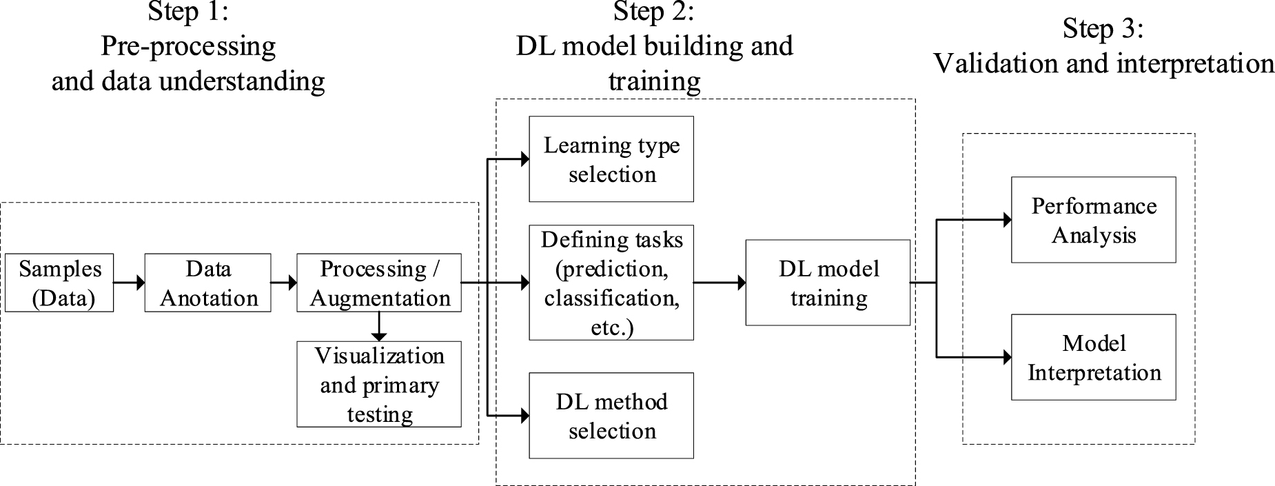
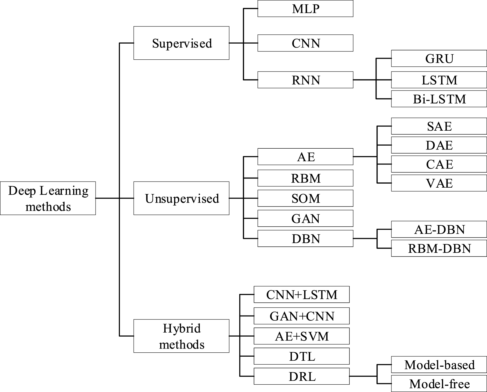
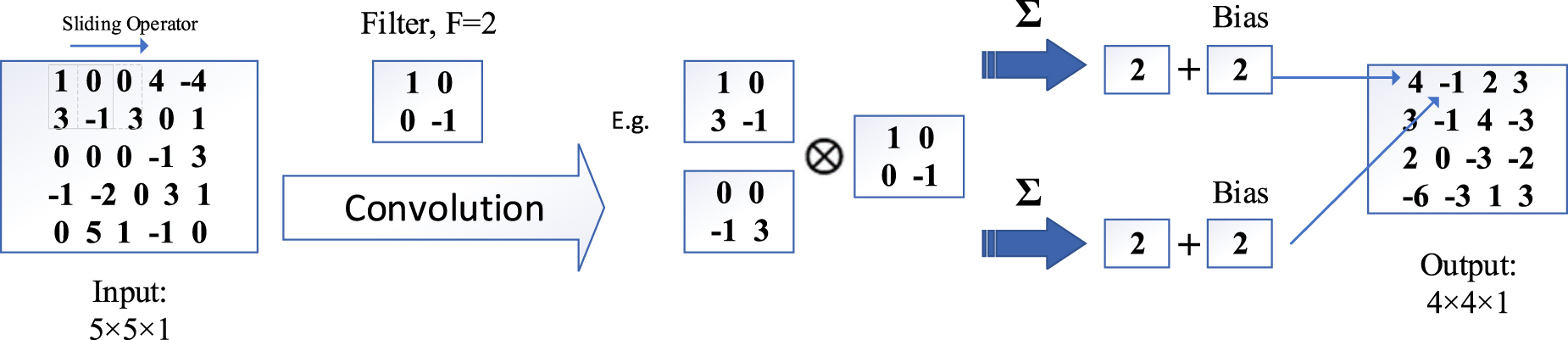
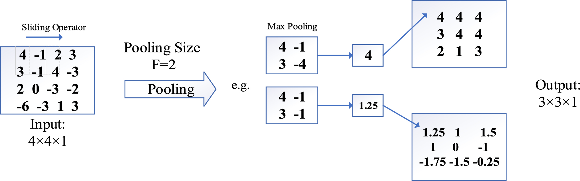
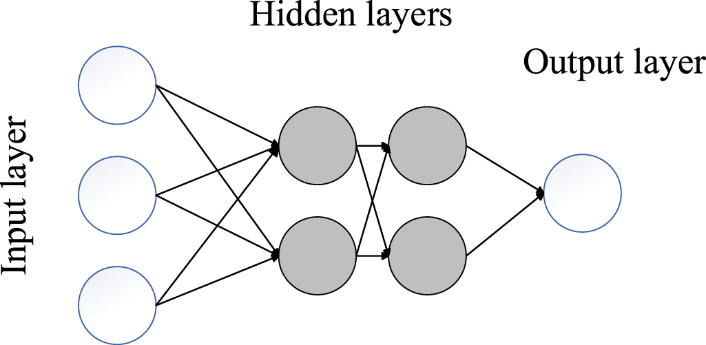
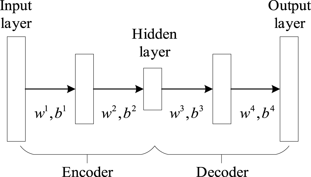
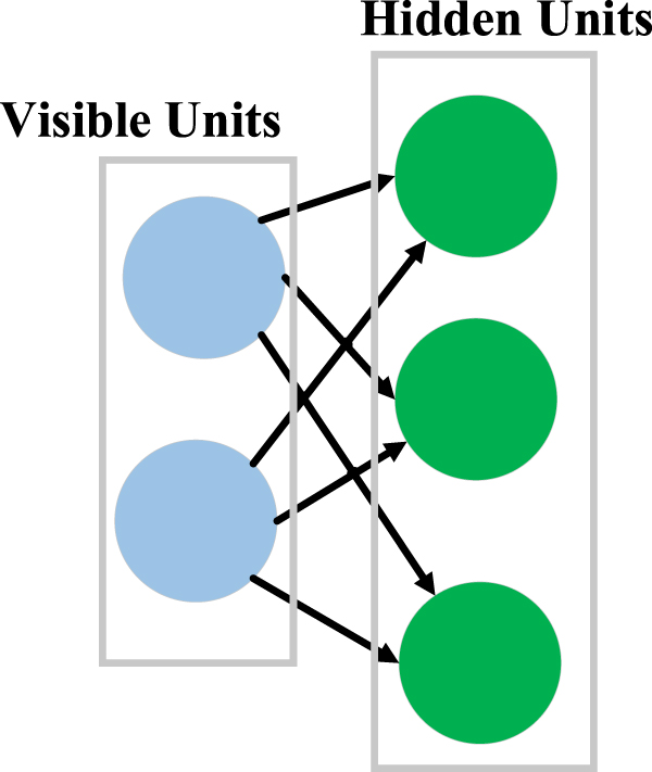
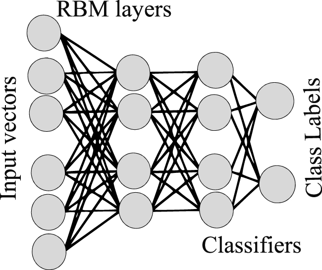
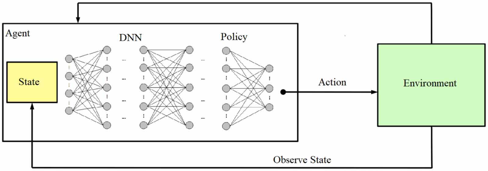
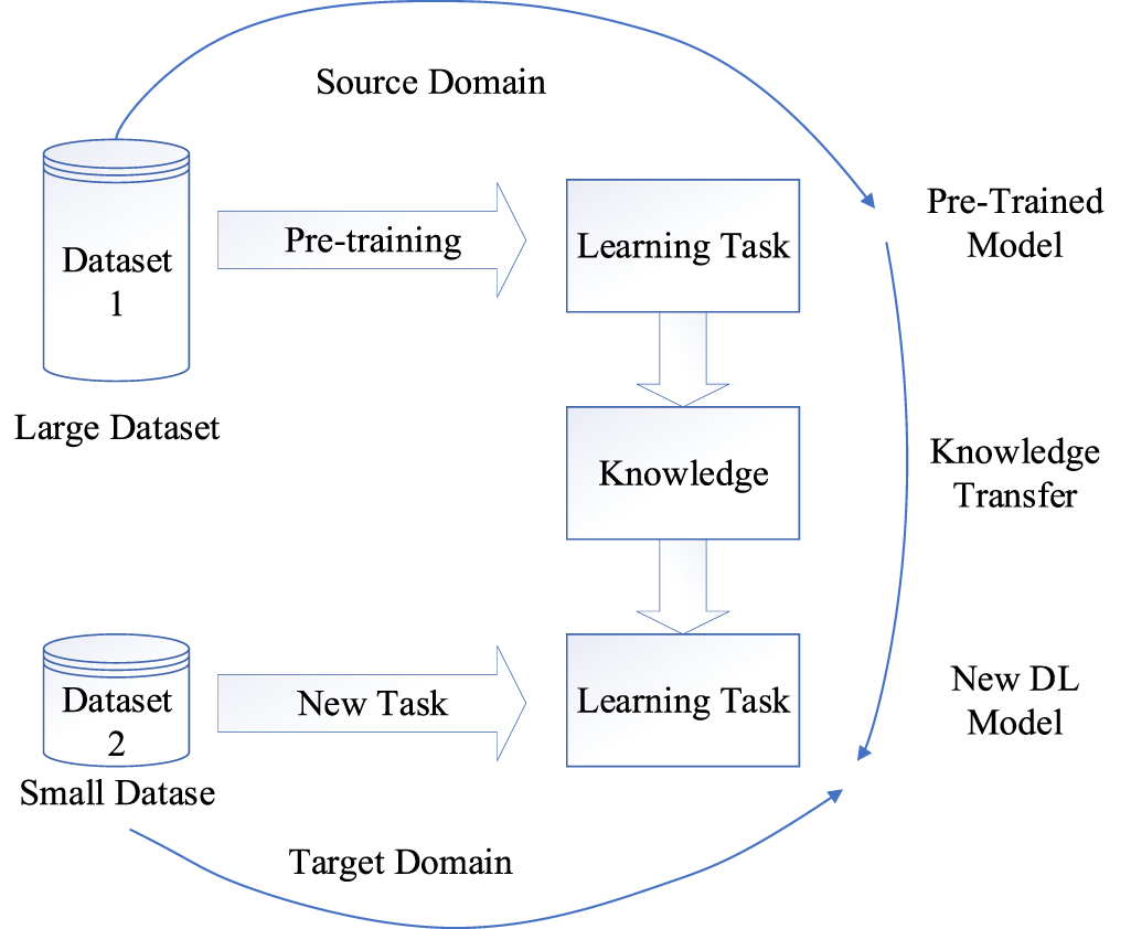
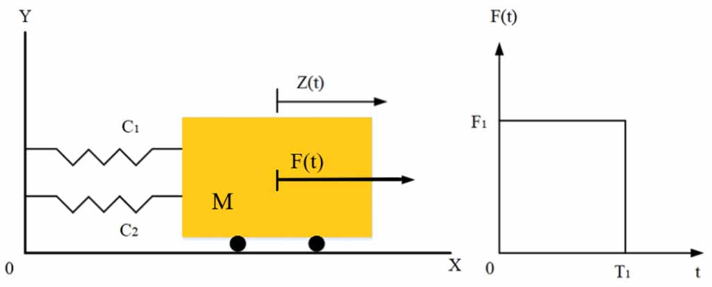
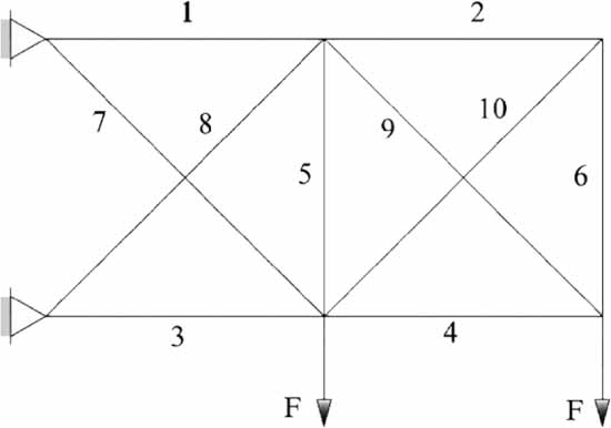
Figure 21. Schematic of a 23-bar truss structure.
Download figure:
Standard image High-resolution image
Table 7. Efficiency and accuracy of results for 23-bar planar truss structure.
| Method | Avg. error of  (%) (%) | Avg. number of calls |
|---|---|---|
| MLP | 14.33 | 250 |
| RNN | 13.23 | 400 |
| CNN | 6.84 | 54.2 |
| LSTM | 1.1 | 66 |
It is valuable to mention that this comparison also requires subtle attention to the SRA problem details. For example, it is mentioned in [13, 22] that altering a constant parameter of the PF can change the failure function significantly, affecting the final results' efficiency and accuracy.
6. Future trends
Here we have reviewed papers that have used different DL-based methods for various SRA problems. Based on the reviewed articles in this manuscript, several topics can show increasing demand and form the future trend of SRA studies. Improving surrogate models' formulation and optimizing the number of sample points are two topics that have received attention as they can help reduce computational time. Studying high-dimensional problems and time-varying reliability and the methods capable of performing real-time SRA are other areas of research in the SRA field that require more attention in the future. Towards those topics, new ML/DL-based methods may also need to be developed. In this section, we go through the mentioned trends more deeply.
6.1. Surrogate models' formulation
As mentioned, regarding computational power growth, DL-based methods have attracted more attention for the formulation of surrogate models in SRA. For example, in the MLP area, the deep MLP with two or more hidden layers exhibits high performance than the shallow MLP or even some other surrogate models. It can allow for more elaborate adaptations to the problem by adjusting its architecture, for example, the number of hidden layers, the number of hidden neurons and the activation functions. It would be interesting to study the role of different layers so as to reduce the number of LSF calls or make it more flexible to adapt various types of LSFs [22]. Besides, DL combined with other methods has shown great potential in saving computational time. Hybrid models, or ensembles, have become a research focus in recent years.
For now, high-dimensional LSFs often occur in the reliability analysis of many engineering scenarios, which proposes a challenge for researchers. For the merit of constructing a low-dimensional latent space in an auto-supervised way, AE is mainly utilized to reduce the dimensionality to alleviate the curse of dimensionality in reliability analysis. However, in the whole procedure of reliability analysis, this work is usually an early step and also needs large-scale training data. In future work, how to optimize the entire architecture based on AE for reliability analysis to improve the accuracy and reduce computational costs need further investigation. Also, GAN has the merit of generating real-like data from random noise variables and making the distribution of the real-like data more similar to that of the real data. Therefore, it is mainly used as a sampling method for reliability analysis to learn and sample from high-dimensional distributions or expand the sample set. In future work, the performance of GAN as a novel sampling method for reliability analysis needs more validation in different high-dimensional scenarios of engineering applications.
6.2. High-dimensional problems
One of the main difficulties in structural reliability problems is to deal with SRA problems of high-dimension systems. The reviewed studies reveal that the accurateness of some techniques is strongly related to the dimension of SRA inputs. In this regard, researchers are more devoted to studying this issue to apply methods to enhance the accuracy, efficiency, and robustness of the method in dealing with high-dimensional SRA problems. In general, DTL and DRL have shown good performance when dealing with inputs with high dimensions [139], which is desirable for complicated systems' SRA in the future. Moreover, enhanced versions of other methods can deliver comparable or superior accuracy. For instance, the new MLP-based method in [22] has achieved outstanding accuracy in SRA of a high-dimensional structural system.
6.3. Time-varying and real-time SRA
An important trend in the future of structural reliability problems is time-varying SRA. One of the key challenges of time-varying SRA is the required computational effort. Recent updates of the LSTM method (such [108, 110, 114]) and MLP-based methods such as [44] have been proposed to estimate time-varying PoF. The combination of some approaches has also offered good performance for time-varying SRA. Another future trend is the simultaneous application of some time-varying reliability analysis methods with DL-based approaches together. For example, the use of DL methods and the probability density evolution method has presented an excellent result for time-varying reliability analysis [149].
Those techniques that can perform real-time or online SRA [22] considering uncertainties from different sources [143], structures with multiple failure modes, and SRA problems with spatially varying parameters (such as [150]), are some other new fields of study in the structural reliability field that can be investigated and be upgraded in the next years. Moreover, automation in data annotation is a trend which shows increasing demand regarding the increasing amount of data analysis power. Nevertheless, data annotation techniques, such as tagging and categorization of large-scale raw data, are essential for constructing discriminative DL-based models. A method capable of intelligent data annotation, mainly for large-scale datasets, can be more efficient and minimize human dependency, saving a lot of time and money. Therefore, an effective data examination and annotation method or designing an efficient unsupervised DL-based method can be one of the main research areas of study in the upcoming years in the field of DL-based SRA. Moreover, DL-based models may become valueless or low-accuracy if the data is corrupt, such as sparsity in the data, low-quality (e.g. high noise), ambiguous values, imbalance values, immaterial features, inconsistency of data, insufficient data, and so on. Therefore, DL-based models also need to familiarise themselves with such growing issues in data collection to become effective for real-time applications.
6.4. Other possible methods for future SRA
As mentioned, regarding the emerging development of DL techniques, DL-based SRA has also made significant progress in recent years. In this sense, there are novel SL-based methods that have the potential to be used in SRA to shape its development in the coming years, here we list some of those methods:
Multi-modal data fusion: many SRA tasks require integrating data from multiple sources, such as sensors, images, and numerical simulations. In the future, DL models that can effectively fuse multi-modal data are likely to become more common, enabling more accurate and comprehensive analyses.
Graph NNs (GNNs): GNNs are a type of DL model that can operate on graph-structured data, such as the connectivity between components in a complex system. GNNs have shown great promise in various domains, and they are likely to become more widely used in SRA as the complexity of systems increases.
Explainable AI: as DL models become more complex, there is an increasing need for techniques that can help explain their decisions. Explainable AI techniques, such as attention mechanisms and decision trees, are likely to become more prevalent in SRA to help identify critical factors for SRA.
Adversarial attacks: adversarial attacks are a type of DL algorithm in which an attacker machine deliberately manipulates the input data to cause a DL model to misclassify it. As DL models become more widely used in critical applications, such as SRA, there is an increasing need to develop models that are resilient to adversarial attacks.
Self-supervised learning: self-supervised learning is a type of DL that uses unsupervised methods to learn from data without explicit labels. This approach is becoming more popular in various domains and is likely to be used in SRA to reduce the need for labelled training data.
Edge computing: many SRA tasks require real-time or near-real-time analysis of data from sensors or other sources. Edge computing, which involves performing computations at the edge of a network, is likely to become more widely used in SRA to enable faster and more efficient analysis of data.
In summary, DL-based SRA is likely to see continued growth and innovation in the coming years, with trends towards novel DL algorithms. These advances are likely to improve the accuracy, efficiency, and effectiveness of SRA, enabling safer and more reliable structures.
7. Conclusions
This article particularized on the trending methods and ideas in the DL-based methods in SRA. The reviewed studies in this survey cover the studies on structural reliability since introducing the concept of AI into this field with a focus on more recent works. Considering current trends in mechanical and civil engineering, it is evident that the need for cost-effective and light-weight structures has encouraged researchers to look for methods to increase SRA's accuracy. Although ML-based techniques have been applied to achieve this goal, they do not perform well when dealing with high-dimensional and nonlinear problems. Accordingly, DL-based methods have been introduced to SRA problems to deal with the complexity and nonlinearity of structures. In this paper, various deep-learning-based methods are categorized into three major sections that are supervised, unsupervised and hybrid methods and have been reviewed. The review reveals that the principal shared advantage of DL-based models is increasing accuracy while maintaining the computational cost within an acceptable margin.
In this paper, we have presented a taxonomy for DL-based SRA methods. In our review study, we have considered deep networks for supervised, unsupervised, and hybrid learning that can be used to solve various real-world issues according to the nature of the problems. Our comparative study has revealed that on average Hybrid methods such as DTL and RL can provide the least average number of calls for high-dimensional problems, and their estimation error also falls under 5% for most of the applications, while they are not very computationally efficient for a less complicated system. When dealing with systems with lower dimensions and less uncertainty, supervised methods such as MLP has usually provided a minor estimation error (under 1%) with an acceptable average number of calls. Unsupervised methods need a proper amount of training data to deliver proper accuracy. For example, AE have shown an estimation error of under 5% for SRA when having an average number of calls of around one hundred. Regarding the reviewed studies in this article, it is understood that the developing need for fast and accurate SRA methods, apparently future SRA methods should align with the use of different AI-based approaches as well as the combination of other methods with ML/DL-based techniques. Furthermore, physics-informed DL techniques integrate data and mathematical physics models, even in partially understood, uncertain and high-dimensional contexts, which has shown a growing interest in recent years.
Acknowledgments
This study is supported by the Natural Sciences and Engineering Research Council of Canada (Grant No. RGPIN-2019-05361), the Research Manitoba New Investigator Operating Grant, the University Research Grants Program (URGP), the Mitacs Lab2Market Program, the China Scholarship Council, and the China Postdoctoral Science Foundation (Grant No. 2022M711808).
Data availability statement
All data that support the findings of this study are included within the article (and any supplementary files).